Dealing with Sample Selection Issues

by trouille scientist, moderator, admin

Hi all (warning, long post, but worth the read, with requests/next steps included).

First, I’m so glad to be back in the discussion. I have not been able to contribute due to medical issues for the past 4 weeks. All is well now (thankfully!) and I can be back in the conversation. I have spent the last few days catching up on the posts of this past month. I've been so impressed with what you all have been finding, your sophistication with the tools and statistics, and your persistence in the absence of input while I've been ill. Thank you all.

There have been a number of interesting results, including mass-dependent merger fractions and here, environment effects, and the role of AGN and here and here.

There are also important questions about the quench and control samples, contaminants, and selection effects (e.g., here and here and here and here.

In order to move forward with confidence, let’s face these questions head on and come to a consensus on a final sample to work with. In re-reading the quenchtalk posts and reviewing the literature, the first step is for us to revisit applying a redshift and magnitude cut to the quench sample.

I thought it'd be helpful to bring the above figure back again here. The legend tells you what each color refers to. Red is for sources with absolute magnitudes brighter than -21.5. Yes, abs_mag is annoyingly confusing in that the more negative, the brighter the source. The red sources are also the most massive sources in the sample (as shown by where they lie in the y-axis). Brighter equals More Massive. That makes sense.

The plot helps us see why Wong et al. (2012) used an absolute magnitude in the Z-band cut of -19.5. Sources fainter than that (the blue in the plot) do not fill across the X-axis direction.

You can also see why Wong et al. (2012) put a redshift cut as well. They use a redshift cut of GT 0.02 and LT 0.05, which is shown by the vertical dashed lines.

If you consider the plot without the blue sources, it seems that we can push to slightly higher redshifts than 0.05 and still feel comfortable with our sample (in terms of how it covers the parameter space). For example, redshifts between 0.02 and 0.08 seem to have reasonable coverage for sources with Z_abs brighter than -19.5.

By applying z=0.02-0.08 and z_mag LT -19.5, we keep 778 sources in the Quench sample (of the original 3002). For the matching revised control sample, pick out the matching control sources to these Quench sources. I’ve provided a list here with the objIDs for the Quench and their matching Control source. It’s cleanest to identify the revised Control sample in this way. (See this post for a reminder on how the Controls are selected in the first place). If there would be a more helpful way of sharing which Controls go with which Quench sources, please let me know.

What now? There are 2 clear steps to take:

#1 – Revisit our results with this stricter sample selection applied. Do we still get statistically significant results?

For starters, Jules – can you give this a try for your merger fraction versus mass plots? Mlpeck – can you see if environmental effects can be seen? Jean or Mlpeck – can you replot the Quench and Control BPT diagrams for this sample?

#2 - Identify if any problematic sources are still in this stricter sample selection of 778 Quench and 778 Control sources. As done previously, let’s group the remaining problematic sources into categories and list their ObjIDs. That way we can make it very clear in the article why we have done any additional removal of sources (if we find that we need to).

Jean, I’ve been impressed with your posts on this topic and attention to detail. Could you take the lead on this? Zutopian, are you still with us? Could you join her in this?

Posted December 2, 2013 7:50 PM
by zutopian

Welcome back! I am pleased to hear, that your state of health is well again!
Yes, I am still here, but there is just tiny participation by me. Anyway. It is fine, that the other volunteers did interesting work.
Interestingly, I communicated about a related topic with Jean by PM today. I would like to work with her, if she is interested, but actually I haven't
the qualification to help her. Anyway. I am going to discuss with her by PM about this matter.

Posted December 2, 2013 11:33 PM
by mlpeck in response to trouille's comment.

Laura:

I hope your medical issues weren't too serious and you're better now.

Regardless of what we decide to analyze in detail one thing I'd suggest is that the quench catalog be published more or less in its entirety. Personally I'd only toss the couple of objects that are isolated stars, and would specifically leave in very nearby objects that are just tiny pieces of galaxies. There's a reason to include some specific nearby objects that I'll try to get to later.

Some other reasons are that the catalog may be a valuable resource for followup work, and the methodology for sample selection appears to be novel and possibly worth applying to other projects. There was an interesting paper posted on arxiv last week that I noted in the background reading section, and I'll quote a paragraph from the conclusion again here:

The absorption features in the nucleus of NGC 1266 indicate the
presence of a non-negligible fraction of model-derived A/K fraction of
NGC 1266 of 2.1 would lead it to be classified as post-starburst in
SDSS, but previous studies have likely failed to recognize the post-
starburst nature of NGC 1266 due to the presence of strong ionized gas
emission. However, as Davis et al. (2012) demon- strated, the ionized
gas in NGC 1266 is most likely the re- sult of shocks associated with
the outflow rather than SF. NGC 1266-like post-starbursts may be
rejected by standard post-starburst searches due to the presence of
the ionized gas emission, and it is therefore imperative to expand the
search for post-starburst candidates to include galaxies with shock-
like line ratios.

Source: Alatalo et al. (http://arxiv.org/abs/1311.6469). While the lack of selection against emission lines may have produced some false positives the sample undoubtedly contains genuinely quenched systems that would probably not have passed through other filters.

Posted December 3, 2013 3:06 PM
by JeanTate in response to trouille's comment.

Welcome back Laura; we missed you. Like zutopian and mlpeck (and, undoubtedly jules and ChrisMolloy, the only others still active as far as I know), I hope you are now well.

I'm very happy with your suggested two steps; it provides a clear focus and goals that I (speaking purely selfishly) can get my head around. Depending on what we find, it should also provide a good foundation from which to explore the other ~2200 QS objects later.

Jean, I’ve been impressed with your posts on this topic and attention to detail. Could you take the lead on this?

Wow! Thanks! In principle, yes, I'd be happy to. But I'd like to read - and respond to - all the other posts you wrote yesterday (last ~24 hours) before committing. I'd also like to hear from jules and ChrisMolloy (and anyone else who's still with us). Above all though, I'd like for us all to seriously consider/discuss mlpeck's alternative suggestion (I'll be responding directly in a bit).

I'm also quite puzzled about why no other SCIENTIST has posted anything; surely they're still reading what's posted? Especially Ivy Wong ... it feels so, um, cold to refer to her as Wong et al. (2012) when she's posted here, with what I think are very helpful and interesting points. Or is this just normal?

Last: the 'jules bug' seems to have bitten me (or my ISP) 😦 I'm having serious internet connection problems, sometimes slow, sometimes quite OK, sometimes completely down; all for no apparent reason or warning (I lost a long post I'd prepared; all major/content-heavy stuff will be prepared offline from now on!). So if I don't seem to be responding in a timely fashion, that's likely why.

Posted December 3, 2013 4:17 PM
by jules moderator

Hi Laura - really good to hear that you are well and back with us! I have already made a start on the merger fraction versus mass plots (adding in redshift cuts) but have been using the same sample size I used previously. No matter - I can adapt and use your new smaller samples. However, I can't open the .tab file you link to. Any ideas?

Otherwise, I suppose I (or anyone else!) could just filter the tables in Tools as you suggest ( z=0.02-0.08 and z_mag LT -19.5).

Sorry to hear you've caught my internet bug Jean - it's very persistent. 😦 Hope you find and rectify the fault soon. I still have intermittent problems and I'm finding Tools is particularly slow at the moment.

Posted December 3, 2013 11:50 PM
by JeanTate in response to jules's comment.

I can't open the .tab file you link to. Any ideas?

It's just a text file, consisting of two columns - of fixed width - and 3002 rows. Each column is an 18-digit number, the DR7 ObjId of a QS (first column) and matching QC one (second). The columns are separated by (two?) spaces, or perhaps a tab.

There are many ways you can open this; here are two:
- edit the file name so that the extension is .csv or .txt instead of .tab (don't do this unless you're comfortable with it! Also make sure you have a copy somewhere else, just in case things go horribly wrong)
- open the file with a 'vanilla' text app, e.g. WordPad (if you have a Windows machine), then save it as a .txt or .csv file
If you open it in a speadsheet, make sure that you require the two columns be 'text'! This is very important!! Most spreadsheets cannot handle 18-digit integers (or at least, not without special treatment) ... they will drop the last three (or so) digits, but keep it as a ~10^18 number (i.e. convert it from an integer to a real). However, these objects are IDs, not numbers, so you need to keep them as text strings.

If none of this works for you, perhaps you could tell us what OS you have?

Posted December 4, 2013 3:22 PM
by jules moderator

Got it - thanks Jean. Opened in Excel fine. (Windows Vista btw)

Posted December 4, 2013 4:41 PM
by JeanTate in response to jules's comment.

Glad to hear it.

I have just finished making a cross-ID table, which matches the DR7 ObjIds with the AGS000... uids. For QS it was pretty simple; for QC it was not ... The v3 QC catalog contains truncated ObjIds (last two or three digits zero; some rounding), so I had to use the v2 one. Unfortunately, v2 contains the duplicates which were removed in v3, and none of their replacements. But I think have a clean table. The table also contains the (RA, Dec) coordinates and redshifts. One sanity check I did was to confirm that the redshifts of the matched QC objects differ by no more than 0.02 (either way) from the QS ones (they do, match that is). Some of the RA values - in QC (I already fixed the QS ones) are given to only 4 significant digits (after the decimal point); this may not be enough to locate the center of the spectroscopic fiber precisely enough. If not, then there's some more work to be done.

Posted December 4, 2013 5:58 PM
by ChrisMolloy

Hi Laura, Good to have you back and I hope you are well now. I've just about finished a look at some aspects of the asymmetrical galaxies and will post hopefully tomorrow. Not based on cuts but will amend for this later. I want to see what differences similarities there are. Trying to track down a quote at the moment which I've lost. Hopefully will find soon.

Posted December 5, 2013 11:41 AM
by jules moderator

Hi Chris! Good to hear from you. Looking forward to seeing your results. I'm also planning to post something I've been working on fairly soon before I embark on the reduced 778 sample. Talking of which.....filtering QS down to the 778 galaxies is easy. Anybody know of a quick and easy way to come up with a matched QC set in Tools? I can think of a long winded way but I'm hoping I've missed the obvious here! 😄

Posted December 5, 2013 4:13 PM
by JeanTate in response to jules's comment.

Anybody know of a quick and easy way to come up with a matched QC set in Tools?

An exact match, no, I can't think of how to do that. An inexact match that you could possibly tweak would be to cut QC on redshift and z_absmag.

Posted December 5, 2013 6:34 PM
by JeanTate in response to mlpeck's comment.

suggest [..] that the quench catalog be published more or less in its entirety ...

I think you're right, mlpeck. Perhaps we could work on doing that in parallel with the analysis Laura proposed? After all, there's no reason that just one paper should be published, nor that we can't multi-task 😉

Suggestion for a small 'value-add' to publication of QS catalog: several - possibly a dozen or so - QS objects are in galaxies where there is more than one SDSS spectrum (of different regions, not just multiple spectra centered on the same (RA, Dec)); add in those where two (or more!) galaxies in a merger each have SDSS spectra, and some quick conclusions should be possible. Oh, and we even have a galaxy with two QS objects in it, quite distinct/different regions! 😮 😄

Posted December 5, 2013 6:45 PM
by mlpeck

I haven't given up. I just spent two days making a 2 segment domestic flight and I've had some issues accessing data on my laptop.

First, I get 792 objects with Laura's proposed magnitude and redshift cuts. I'm just using the K-corrected z band absolute magnitudes and redshifts in the data table downloaded from tools. But, no matter.

I'd also like to suggest slightly different cuts. Here is a plot of z band absolute magnitude against redshift (note the latter is on a log scale):

If the magnitude limit is decreased to -20 and the upper redshift limit is increased to z=0.1 the sample will still be volume limited, in fact to a somewhat better approximation than Laura's proposed redshift cuts. This will increase the analyzed sample to 1149 -- 93 are lost to the lower magnitude limit but many more are gained in the redshift bin 0.08 < z < 0.1.

Either way the spectroscopically starforming fraction is going to increase considerably compared to the full sample while the "unclassifieds" will decrease. Everything else maintains about the same proportions in the BPT diagram:
```
table(bpt.quench[sub1.quench])

  0   1   2   3   4 
 86 430 145  48  83 
> table(bpt.quench[sub2.quench])

  0   1   2   3   4 
157 541 247  82 122 
> table(bpt.quench[sub1.quench])/792

         0          1          2          3          4 
0.10858586 0.54292929 0.18308081 0.06060606 0.10479798 
> table(bpt.quench[sub2.quench])/1149

         0          1          2          3          4 
0.13664056 0.47084421 0.21496954 0.07136641 0.10617929 
```
I haven't looked at any other properties of the proposed trimmed sample yet, and may not have time to do much for a while. I'm also not going to participate in any outlier chasing threads.

It seems to me that what most needs explaining is why there are so many starforming galaxies in the "quench" sample, and that needs explaining even more if we limit the analyzed redshift range.

Posted December 6, 2013 5:46 PM
by JeanTate in response to mlpeck's comment.

First, I get 792 objects with Laura's proposed magnitude and redshift cuts.

The difference - 14 objects - is those with log_mass = -1 😃

Posted December 6, 2013 9:45 PM
by mlpeck in response to JeanTate's comment.

Oh, right. Had my advice to use DR8+ stellar mass estimates been acted on none of those would be missing, nor would there be any in the suggested expanded sample.

Posted December 6, 2013 11:34 PM
by trouille scientist, moderator, admin in response to mlpeck's comment.

Yes, that makes a lot of sense --- to post the entire Quench catalog and then include flags to indicate problematic sources. There is a lot of precedence for that type of approach. Then for our science results, we would make it clear what sample selection we apply so that any follow up studies can recreate our results.

Posted December 9, 2013 8:25 PM
by jules moderator

I get 808 items. Clearly I am doing something wrong. I am working in Tools with the following filters:

filter .'Log Mass' !=-1

filter .z_absmag<-19.5

filter .redshift<0.08

filter .redshift>0.02

Help!

(And thanks in advance.)

Posted December 9, 2013 9:49 PM
by JeanTate in response to jules's comment.

You're applying this to the QS catalog (and not the QC one), right?

It shouldn't make a difference, but what happens when you apply the filters in reverse? I.e. start with z > 0.02, then z < 0.08, then ...

Posted December 10, 2013 12:07 AM
by trouille scientist, moderator, admin in response to jules's comment.

However, I can't open the .tab file you link to.

Ach, sorry. Try this file instead (https://docs.google.com/spreadsheet/ccc?key=0AgvyjftFXUCddEtQVmJBbGxrWU4yWEZZX1VvRVdjTmc #gid=0). I forgot that .tab files aren't as easy to open in Excel and other spreadsheet programs as .csv files. With this google spreadsheet, you should be able to download the data or copy and paste it to any program.

Posted December 10, 2013 12:11 AM
by trouille scientist, moderator, admin in response to JeanTate's comment.

Awesome Jean. Just responded about another way to get the .tab data from a Google spreadsheet, but I much prefer your instructions. Need to learn to read a whole thread first!

Could you share the...

I have just finished making a cross-ID table, which matches the DR7 ObjIds with the AGS000... uids.

with us? That would be really useful to work with.

Posted December 10, 2013 12:25 AM
by trouille scientist, moderator, admin in response to jules's comment.

Jules post: I get 808 items... with the following filters:filter .'Log Mass' !=-1, filter .z_absmag<-19.5, filter .redshift<0.08, filter .redshift>0.02

Hey Jules,

I did those filters on the Quench sample and got 778 sources in Tools. This is my Dashboard. http://tools.zooniverse.org/#/dashboards/galaxy_zoo_starburst/52a6611c5b6a1304a0000027

Something funky is going on with your attempt. If you share your Dashboard, I can definitely look.

A more intractable problem is that you can't overplot in Tools (i.e., plot the Quench results with the Control sample results overplotted in the same plot) and, like Jean, I can't think of a good way of getting the right Control sample matched to this Quench restricted sample.

This (and other discussions) has made me think that for future Quench-style projects (if you all think it's a good idea to try this again at a future date), we might want to consider bringing in learning Python (as Mlpeck has suggested) early-ish on in the project. So that when we get to this stage, people have the tools that can actually allow them to do what they need to do (in particular, statistical analysis, binned data, etc.).

Tools will still have an important role of being a user-friendly* introductory data analysis platform for people to use. But the idea would be to transition to something more sophisticated over the time of the project.

What do you all think?

BTW, totally OK not to respond to the 2nd part of this post and just focus on the analysis at hand!

*I know, it wasn't so user-friendly at the start of Quench... I do think it's better now, though there's still work to be done.

Posted December 10, 2013 12:34 AM
by trouille scientist, moderator, admin in response to mlpeck's comment.

mlpeck wrote: Oh, right. Had my advice to use DR8+ stellar mass estimates been acted on none of those would be missing, nor would there be any in the suggested expanded sample.

Good reminder. Mlpeck or Jean -- could you possibly make a google spreadsheet with the first column showing the ObjIDs of the 14 objects and the 2nd column with their mass from DR8. That would be really useful. I know Mlpeck that I can get them from the casjobs that you created, which I will do, but this will be a good way to make those easily accessible to all.

Posted December 10, 2013 12:44 AM
by JeanTate in response to trouille's comment.

I've never used Google Spreadsheet in this way before, so I hope this works ...

If you click this link, you should get a document (Google spreadsheet) called QSQCIDs. In addition to the pairs of ObjIds and uids, there's also the (RA, Dec) for each pair, and the redshifts. Some cells are colored (orange, yellow); ignore this (it had some meaning in an earlier file, but none here). The column "Ref" is unnecessary (it's a safety feature, in case I messed up the sorting). Questions? Just ask!

Posted December 10, 2013 8:18 AM
by jules moderator

Cool - thanks Jean!

Posted December 10, 2013 4:18 PM
by JeanTate

Thanks jules. I guess you checked it out, and found that you were able to open/download it OK? I got a PM from another zooite about this, and it seems that it does, in fact, work. Yay!

Emboldened, I created a similar Google spreadsheet, just for 'the 778'; it is here. Would someone please check it out, and confirm that it works? Of course, it works for me, but I'm the author, so that's not a fair test.

This new spreadsheet has a few more columns; I hope that you find them helpful.

Posted December 10, 2013 4:36 PM
by jules moderator

OK - bad schoolgirl error - I used QC rather than QS. Silly dashboard renaming error. I've quadruple checked that all my work so far uses the appropriate datasets and all is fine!

And I now have the correct reduced sample number. 😄

Jean - the 778 spreadsheet works just fine.

Posted December 10, 2013 4:46 PM
by mlpeck in response to trouille's comment.

Good reminder. Mlpeck or Jean -- could you possibly make a google
spreadsheet with the first column showing the ObjIDs of the 14 objects
and the 2nd column with their mass from DR8. That would be really
useful. I know Mlpeck that I can get them from the casjobs that you
created, which I will do, but this will be a good way to make those
easily accessible to all.

I can't immediately figure out how to use Google spreadsheets and don't have time to work on it right now. My dropbox account has a CSV file with DR8+ mass estimates, Lick Hδ index values, specObjId's and some other data for all 3000 objects in my data set. I'm afraid you'll have to work out which are the missing 2 objects but the ordering should otherwise be the same.

Here is the link: https://www.dropbox.com/s/js6oh9dctavak5o/qmasshd.csv.

The column with the updated mass estimates is "lgm_tot_p50" and the original "log_mass" values are included for comparison. There are a couple missing values indicated by the string "NA".

What did you think of my suggestion to adjust the redshift and magnitude cuts a little bit?

To save you searching back through this thread the suggestion was to increase the redshift limit to z=0.1 and decrease the magnitude limit to Z = -20. This will increase the analyzed sample size to ~ 1150.

Posted December 10, 2013 5:40 PM
by JeanTate in response to mlpeck's comment.

The tab/sheet "missing" - in this Google spreadsheet - contains the data (I hope); i.e. the estimated log_mass of the 14 QS objects in 'the 778', for which log_mass is given as -1 in v4 of the QS catalog.

The two "NA" are AGS00000fb (which has a log_mass of 12.5209 in the QS catalog) and AGS000017k, whose log_mass is 'missing' (it is also the QS object with the highest redshift, by quite a ways).

Posted December 10, 2013 7:27 PM
by jules moderator

I see that too - estimated log mass being in the column headed " lgm_tot_p50." Very helpful. Thanks again Jean.

Posted December 11, 2013 12:00 AM
by JeanTate in response to trouille's comment.

This (and other discussions) has made me think that for future Quench-style projects (if you all think it's a good idea to try this again at a future date), we might want to consider bringing in learning Python (as Mlpeck has suggested) early-ish on in the project. So that when we get to this stage, people have the tools that can actually allow them to do what they need to do (in particular, statistical analysis, binned data, etc.).

Tools will still have an important role of being a user-friendly* introductory data analysis platform for people to use. But the idea would be to transition to something more sophisticated over the time of the project.

What do you all think?

The main thing I think is ... we should have a whole separate discussion on this topic!

Here are a few, rather random, of my thoughts:
- a 'research grade' project will likely require more than Tools and/or Google Spreadsheet, at least in part
- while Python is awesome, unless there's a way to do all Python-based analyses online somehow, or get it to run reliably under Windows, using it will rather drastically cut the number of zooites who'd even consider taking part
- Tools has great potential ... but it's also got rather a lot of show-stopper shortcomings (so far as a project like Quench is concerned); how realistic is it to expect that these can be overcome?
- the major 'lessons learned' from this project are rather different than 'the toolkit we chose was less than ideal'
Posted December 11, 2013 3:48 PM
by JeanTate in response to mlpeck's comment.

What did you think of my suggestion to adjust the redshift and magnitude cuts a little bit?

To save you searching back through this thread the suggestion was to increase the redshift limit to z=0.1 and decrease the magnitude limit to Z = -20. This will increase the analyzed sample size to ~ 1150.

Hope you don't mind if I also answer this ... an upper redshift limit of ~0.085 has much to commend it, in terms of SDSS spectroscopy completeness, being genuinely volume-limited, and so on. I started to look into this some time ago, but didn't get far enough to write anything solid. I will try to pull it all together today or tomorrow ...

Posted December 11, 2013 3:54 PM
by zutopian in response to JeanTate's comment.

Thanks for posting the link of the google spreadsheet "778 QS/QC galaxies".
I have a question concerning BPT types.: There are given numbers from 1 to 7. What does each number stand for?

Posted December 12, 2013 6:22 AM
by jules moderator in response to JeanTate's comment.

Re JeanTate's comment concerning incorporating Python into future projects - I think you are right Jean in that this would reduce participation in the analysis stage drastically. In which case Tools needs some work to allow more analysis to be done there.

Posted December 12, 2013 12:19 PM
by JeanTate in response to JeanTate's comment.

I will try to pull it all together today or tomorrow ...

Dividing the ~3k QS objects into redshift bins 0.01 wide, selecting the object with the brightest z_absmag (estimated absolute magnitude, in the k-corrected/'local dust removed', SDSS z-band) and plotting them gives you the blue diamonds. The dark blue line is the 'log' best fit trend line. The orange diamonds are the r-band magnitudes of the faintest sources in each bin, with a minus sign in front so they can be plotted together. The two dotted horizontal lines are at 17.0 (the lower/faint limit for the GZ2 work, sorta) and 17.77 (the lower/faint limit of spectroscopic 'galaxy' targets in DR7)^caveats.

All bins but the last eight have lots of objects, so 'small number selection' effects should be minor for all other bins ... clearly there's a lot more going on! Also, the light blue line is a 'volume limited' one, for a universe assumed to be Euclidean, with a somewhat arbitrary constant.

Perhaps you, mlpeck, can make sense of this (I'm sure all the SCIENTISTs can), but it's got me quite confused ... why are there no intrinsically bright QS objects in bins #3 and #4? Why are there no apparently faint QS objects in so many bins (all the orange diamonds above the '17 mag' line!)? Is this all somehow tied up with there being more Eos at low redshift, and a rising fraction of 'pure AGN' with redshift?

Anyway, back to mlpeck's question: contrary to what I wrote earlier, the data seem to be saying that the proposal is OK, with perhaps a minor edit, that the Z limit be closer to -20.5 (and that Laura's, re 'the 778', be closer to -20).

^caveats I should give links to sources; if anyone wants them, just ask! Also there are 12 QS objects excluded: two are stars (their z_absmags are +ve!); the highest redshift object is waaay off to the right; eight are fainter than 18 (r-band), so well outside the DR7 target range; the last has an r-band mag of 17.85, perhaps I should have left that one in. There's no reason to expect that the faintest z_absmag object in a bin will also be the faintest r-band one (except for bins with few objects), but it often is.

Posted December 12, 2013 9:13 PM
by JeanTate in response to zutopian's comment.

You're very welcome!

I have a question concerning BPT types.: There are given numbers from 1 to 7. What does each number stand for?

Hmm, if you hover your mouse over the two column headings, do you see something like this?
1. AGN
2. SFR
3. composite
4. maybe LINER
5. low Ha SF
6. all em, low S/N
7. >0 null em
8. all null
The first three are the usual BPT regions; the next two are - hopefully! - the same as is given by the DR8 spectroscopic pipeline ("Low S/N AGN" and "Low S/N Star Forming"); the last three are all "Unclassifiable", split into those with four emission lines each with positive flux, those with at least one with positive flux, and those for which all four fluxes are 'null' (i.e. zero or negative).

Posted December 12, 2013 9:24 PM
by mlpeck in response to JeanTate's comment.

If we're going to extend or modify the traditional BPT diagnostic diagram I'd suggest considering the WHAN diagnostic of Cid Fernandes et al. (2010, 2011). It makes use of [N II] and Hα fluxes and equivalent widths and no other lines, which has the disadvantage that more data must be fetched from Casjobs. It may have the advantage of being less ad-hoc than simply relaxing the classification criteria. It certainly has the advantage that many more QS objects become classifiable. By my count 192 out of 3000 would still be classified as passive, while a few hundred would fall in their intriguing "retired galaxy" bin.

Posted December 13, 2013 1:24 AM
by zutopian in response to JeanTate's comment.

I didn't notice, that there is a specification given in the google spreadsheet. Thanks for your comment about those BPT types.
I think, that the quantities for SFR and low Ha SF are puzzling.:
There are however 432 (56%) QS galaxies, which are SFR.There are less QC galaxies, which are SFR.: 357 (46%).
There are however just 3 QS galaxies, which are "low Ha SF". There are 165 QC galaxies, which are "low Ha SF".

Posted December 14, 2013 6:54 AM
by JeanTate in response to zutopian's comment.

Yes, I too found this rather puzzling (see this post, in the Characterizing 'the 778': how do the QS objects differ from the matched/paired QC ones? thread).

Posted December 16, 2013 3:28 PM
by JeanTate in response to mlpeck's comment.

I did not, and do not, intend to extend or modify it; rather simply to use what is already provided by the DR8 spectroscopic pipeline. My categories 6, 7, and 8 were just a way to quickly find objects which may be spectroscopically problematic (e.g. has a 'piece missing', a wavelength range which includes one or more of the four emission lines used), so I could check them.

In trying to track down some examples, I think I found something I've always dreaded: somewhere along the line I messed up a copy/paste or a sort (or something), and now some of my fields for at least some of the objects no longer match 😦 I'll need to go and (re-) check. Thanks to you, and to zutopian, for helping me find this (potential) problem.

Posted December 16, 2013 3:50 PM
by trouille scientist, moderator, admin in response to mlpeck's comment.

I've been meaning to do more justice to mlpeck's post about an alternative cut to the one I proposed. Definitely a good scientific approach to explore different cuts, their impact on our major results and on our sample selection robustness/reliability. Being able to use a larger subsample of the full selection is highly desirable.

Quick question -- do the different colors in your plot map to different colors in the BPT plots you've shared? I"m pretty sure they do but want to be sure they don't map to mass or something else.

Posted December 17, 2013 6:45 PM
by trouille scientist, moderator, admin in response to mlpeck's comment.

Paraphrase of Mlpeck's post: To save you searching back through this thread the suggestion was to increase the redshift limit to z=0.1 and decrease the magnitude limit to Z = -20. This will increase the analyzed sample size to ~ 1150.

In the plots below are the same cuts (Abs_Z LT -20 and redshifts from 0.02 - 0.1).

As Mlpeck mentioned, the more negative the absolute magnitude, the brighter the source. By changing the Z_ABS_Mag limit to -20 (rather than -19.5), you reduce the sample size slightly (by ~93 sources). But by increasing the redshift limit to 0.1, you include hundreds more sources. This is very desirable.

https://vault.it.northwestern.edu/let412/GZQuench/Talk_Images/RedshiftVsMass_wMag_neg20_small.jpg

https://vault.it.northwestern.edu/let412/GZQuench/Talk_Images/RedshiftVsMass_wMag_final_small_9p5.jpg

The axes of the two plots are the same. In the top plot, our final subsample would be just the red objects between the vertical redshift cut lines.

In the bottom plot, the color is the same as in the legend in the top plot. All I've done is get rid of objects above and below the redshift cuts and outside our abs_mag cut. And I've placed an arbitrary horizontal line at mass = 9.5.

The point of the 2nd plot is for us to think about whether by extending the redshift limit to z=0.1, we are introducing a potential sample bias. There is a slight triangular hole where there are few-to-no objects in the bottom right, wedged up against the dotted lines. There are low mass galaxies that live between z=0.08 and z=0.1, but because they are faint, they drop out of our sample selection as we go above z=0.08. What I find encouraging is that the hole in parameter space is small and may not have important impact on our results.

In order to know whether this hole in parameter space does impact our results, I recommend that for all results we share, we share two versions: One with a sample selection that restricts redshift to z=0.02-0.1 and the other with z=0.02-0.08.

The motivation is that mlpeck's subsample is significantly larger than the more redshift-restricted sample. It would be great if we find that we see similar trends with the smaller and larger subsamples. That will allow us to make stronger statements in our article about the robustness of our results.

Posted December 17, 2013 7:57 PM
by trouille scientist, moderator, admin in response to mlpeck's comment.

As for whether to use an Abs_Z cut at -19.5 or -20, I am unsure. If you look at the plot below (I've added back in the ~90 sources with abs_Z between -19.5 and -20, shown in green), they cover similar parameter space as the lower-mass, lower-redshift abs_Z LT -20 sources.

Mlpeck and others, are there additional reasons I should be thinking about for why to remove the abs_Z from -19.5 to -20 sources?

Thanks!

https://vault.it.northwestern.edu/let412/GZQuench/Talk_Images/RedshiftVsMass_wMag_final2_small.jpg

Posted December 17, 2013 8:32 PM
by trouille scientist, moderator, admin

Mlpeck and/or others: Could you make a .csv file available that has all the meta data but cut down to only sources in the subsample you've suggested (Abs_Z LT -20 and redshift between 0.02 and 0.1)? Could you also provide a .csv with the subsample with Abs_Z LT -19.5 and redshift between 0.02 and 0.08?

That way anyone in the group using Excel can more easily work with these latest subsample selections that correctly match the Quench with the Control samples (i.e., remove the Control sample sources that correspond with the Quench sample sources that are removed). Because it's not possible to do this removal in Tools, it'll be really helpful if we provide this.

Definitely include the object IDs in the .csv files. That will help us incorporate what we're learning about problematic sources through Jean et al.'s efforts.

Thanks!!

Posted December 17, 2013 8:47 PM
by trouille scientist, moderator, admin in response to JeanTate's comment.

Although of course not fun to find errors in your workflow, really great to see that discussions between you all led to finding it -- very much part of the scientific process. And definitely repost about these results when you've done your double check -- really useful to be checking how the two samples compare.

Posted December 17, 2013 8:59 PM
by mlpeck in response to trouille's comment.

Quick question -- do the different colors in your plot map to
different colors in the BPT plots you've shared? I"m pretty sure they
do but want to be sure they don't map to mass or something else.

Yes, sorry. I dispense with legends sometimes. The graph I posted way back on page 2 of this topic used the same color coding as in my BPT diagram plots. It's more or less obvious there that the mix of emission line properties changes with redshift - no doubt a selection effect!

As for the specific suggested magnitude and redshift cuts, I was just eyeballing possible alternatives that would still produce something close to a volume limited sample.

Posted December 17, 2013 9:06 PM
by mlpeck

Mlpeck and/or others: Could you make a .csv file available that has
all the meta data but cut down to only sources in the subsample you've
suggested (Abs_Z LT -20 and redshift between 0.02 and 0.1)? Could you
also provide a .csv with the subsample with Abs_Z LT -19.5 and
redshift between 0.02 and 0.08?

Doing this for the quench sample would be no trouble at all, but I'm not sure I can get an exact match of the control sample subset. Here's the problem: the versions I had downloaded had apparently been imported into a spreadsheet and exported again, because the SDSS id's were rounded off to the nearest thousand.

I checked the data tables in tools today (12/18) and that issue has been solved, but the control sample now has just 2,946 rows. Was there a version of the control sample that size? I don't remember.

There's probably a workaround, but it's going to take more effort than just using the cross-reference table you provided as an index.

Posted December 18, 2013 4:56 PM
by mlpeck in response to trouille's comment.

Mlpeck and/or others: Could you make a .csv file available that has
all the meta data but cut down to only sources in the subsample you've
suggested (Abs_Z LT -20 and redshift between 0.02 and 0.1)? Could you
also provide a .csv with the subsample with Abs_Z LT -19.5 and
redshift between 0.02 and 0.08?

I've uploaded CSV files for these two quench sample subsets to my dropbox account.

Subset 1 - .02<z<0.08 & Abs_z< -19.5 https://www.dropbox.com/s/4sdkqbxxzxq3x1a/quench.subset1.csv

Subset 2 - .02<z<0.10 & Abs_z< -20 https://www.dropbox.com/s/ae3w7ebuqevbmio/quench.subset2.csv

I've added 3 columns to both data sets: lick_hd_a and lick_hd_a_err are the Lick Hδ_A absorption line index and error taken from the MPA pipeline, and lgm_tot_p50 is the DR8+ log stellar mass estimate, also from MPA. Feel free to compare these estimates to the log_mass estimates in the original data table. They should be nearly enough identical except for the no longer missing values.

There are 792 entries in subset 1 (including 14 no longer missing mass estimates) and 1149 in subset 2 (including 27 with missing masses in the original data set).

A couple formatting notes. Strings are quoted, including column headers. I think Unix/Linux convention is used for end of lines. The string "NA" is used to denote missing data. Those are scattered throughout. I don't know how these will be handled by spreadsheet programs. LibreOffice Calc seems unconfused -- at least it recognizes the other entries as numeric.

I still don't have an easy way to get a 1 to 1 correspondence of control objects to QS objects. I may save that for Christmas.

Posted December 19, 2013 9:35 PM
by JeanTate in response to trouille's comment.

Quick note for now: I have almost finished a top-to-bottom, very careful re-processing of all the relevant data, starting with the .csv v4 QS and QC catalogs. I did this without looking at any of the files or analyses I'd done before.

The good news in a nutshell: the only differences between 'before' and 'now' are in the field 'BPTtype'. And there are only a few dozen discrepancies in 'the 778' (and ~150 in the whole 3002x2 dataset). This is a great relief.

Along the way I had to address several rather awkward problems, and resolving them was tedious indeed; I'll say more about this in a later post. Also in a later post, I'll look at what the 'BPTtype' differences are, and see if I can understand - and explain - how they came to be.

Finally, I'll be posting links to Google spreadsheet 'cross-ID' files ...

Posted December 19, 2013 11:32 PM
by JeanTate in response to mlpeck's comment.

I have just such a file (actually a pair, one for each of the proposed selections). Once I've checked it (them), I'll be uploading it as a Google spreadsheet, which can be accessed as a .csv, I think (I don't have a site to which I can upload an arbitrary file type, which anyone can access and download)

Posted December 20, 2013 12:56 AM
by JeanTate in response to JeanTate's comment.

Along the way I had to address several rather awkward problems, and resolving them was tedious indeed; I'll say more about this in a later post.

As mlpeck mentioned above, perhaps the thorniest problem is the fact that, in both the v3 and v4 catalogs (both QS and QC), the SDSS DR7 ObjIds have been 'rounded' (someone treated them as ordinary integers, rather than text strings). As I have both the QS and QC v2 (and v1) catalogs - in which the IDs are given in full - I am in a position to match these with their 'uid' (the AGS000... identifiers).

So, for example, AGS0000001 (a QS object) is 587725074458345628 (587725074458345600 in v4), and AGS00002bf (a QC one) is 587739827133939896 (587739827133939800 in v4) ... and from the file Laura posted earlier, we know that these are a QS-QC pair.

Piece of cake, right?

Wrong!

Remember those duplicates? The 13 QC-QC ones (26 objects in all) and the 29 QS-QC ones? They are in v2, but not in v4 (obviously). There's also the QC object with the crazy redshift ... it's in v2 but not in v4. The good news is that there are only 56 of these (=2*13+29+1), and - in almost all cases - only the last three characters (digits) in the (18 character/digit) ObjId text string are affected by truncation¹; it should be possible to find the full ObjId that matches the truncated one. And it is (I did just that). To be sure there were no surprises, I checked each of the 56 'GZ image' webpages, which displays the uid and its matching DR7 ObjId². Tedious? Yes, but at least I was able to confirm that the QC uids matched the DR7 ObjIds!

¹ if you try to match the truncated QC ObjIds (in the v4 catalog) with the full ObjIds (in the .tab file), you'll find a good dozen or so 'ambiguous' cases ... pairs of identical truncated ObjIds, but two distinct full ObjIds (as mlpeck found)

² even though, when you click the View on Sky Server link, you get a DR9 image, and so a 19 character/digit SDSS DR9 ObjId! 😮

Posted December 20, 2013 1:28 AM
by JeanTate in response to mlpeck's comment.

... but the control sample now has just 2,946 rows. Was there a version of the control sample that size? I don't remember.

3002 - 2946 = 56. No, it's not a coincidence.

Posted December 20, 2013 1:34 AM
by JeanTate in response to JeanTate's comment.

Finally, I'll be posting links to Google spreadsheet 'cross-ID' files ...

If you click this link you should get a Google Docs file, QSCXIDv2.csv (please let me know if you can't!).

You should be able to download this, and open it with a spreadsheet app (Excel, OpenOffice Spreadsheet, ...). MAKE SURE YOU MARK the fields "SObjId' and 'CObjId' - the SDSS DR7 ObjIds, which look like 18-digit integers, but aren't - AS TEXT!! If you don't, your spreadsheet will (very likely) think they're integers, and truncate the values, making the last two digits/characters zeros.

The fields are all named in the first row and should all be pretty self-explanatory: if it's got an "S" in it, it refers to the QS (quench) catalog, and if a "C", the QC (control) one.

Everything comes from the v4 catalogs, EXCEPT:
- the SDSS DR7 ObjIds are from the v2 catalogs, PLUS my reconstructions of 'the 56' QC objects (see my posts above)
- the two "BPTtype" fields: these are my own creation, and are explained in detail below
- the "the778" and "the201" fields: in both the values are either 1 ("in") or 9 ("out"), meaning QS objects with redshifts >= 0.02 AND <= 0.08 ('the778") or 0.10 ("the201") AND z_absmag <= -19.5 ('the778") or -20 ("the201") AND log_mass != -1
I will be producing a v3 which will differ from v2, as follows:
- for ~2.5k QS objects, more accurate (RA, Dec) values, courtesy of mlpeck
- replacing log_mass "-1" values with estimates from mlpeck (NOTE: some "-1" objects will remain)
About the 'BPTtype' values:
- 1, 2, and 3 are the types per the traditional diagram: AGN (1), Star forming (2), and Composite (3); see below for the formulae I used
- 4 is "low S/N AGN", per SDSS DR8; see below for the formula I used
- 9 is everything else
Posted December 20, 2013 4:52 PM
by trouille scientist, moderator, admin in response to JeanTate's comment.

I just emailed Ed about this difference (i.e., a different number of Quench vs Control sources in Tools). This is an error. My hope is he can fix the Control sample in Tools today. He or I will post when he does.

In terms of the process -- I give him the meta data tables for all 3002 sources in both the Quench and Control samples. He then puts them into the Tools database (the tables have to be converted into a format that the website can read). For the next Quench, we've talked about changing that set up so that the science team can do the changes ourselves, so there's nothing lost in translation.

Posted December 20, 2013 7:31 PM
by trouille scientist, moderator, admin

Ed just let me know that the Tools Quench tables are back to 3002 sources each.

Posted December 20, 2013 8:47 PM
by JeanTate in response to JeanTate's comment.

The good news in a nutshell: the only differences between 'before' and 'now' are in the field 'BPTtype'. And there are only a few dozen discrepancies in 'the 778' (and ~150 in the whole 3002x2 dataset). This is a great relief.

Along the way I had to address several rather awkward problems, and resolving them was tedious indeed; I'll say more about this in a later post. Also in a later post, I'll look at what the 'BPTtype' differences are, and see if I can understand - and explain - how they came to be.

All but three of the differences (i.e. objects with BPTtypes that, in my top-to-bottom review, are different from what I'd been using) concern BPTtype 5, "low S/N SF". And all these "low S/N SF" assignment differences are due to inconsistent application of the selection criterion. It seems that the reference paper for this BPT classification is Brinchmann et al. 2004¹. In my review I found that I had previously misunderstood - or, perhaps more accurately stated, misapplied - the selection criterion for this class. I now feel that this class is more trouble than it's worth, and will be using only the traditional three classes - AGN, SFR, and Composite - plus "low S/N AGN", and "else/rest/other" from now on.

What about the other three? Well, for two a value of a key parameter is so close to the threshold that in my previous assignments I'd put them on 'the wrong side'. How come? Because instead of letting a formula make the call, I'd simply ranked (sorted) a list and 'cut by eye': all members of the list 'above' the threshold are 'in', all 'below' are 'out'. Trouble is, the numbers displayed are automatically rounded!

The last one - AGS00001y8 - illustrates the importance of doing sensibility checks: blind application of formulae suggests this is a low S/N AGN; however, with an Ha flux of 19333900000, an Hb one of 3283180000, etc, it's obvious that there was a catastrophic failure in the SDSS spectroscopic pipeline. So this object's BPTtype is 'else/rest/other'.

¹ I'm following this SDSS DR8 page

Posted December 21, 2013 2:55 PM
by JeanTate in response to JeanTate's comment.

As I had downloaded a copy of the QC catalog before Laura's post, I was able to compare the "just 2,946 rows" catalog with v4.

If you sort by uid, you find the first 2946 objects match: they go from AGS00002bf to AGS00004ms. In the v4 QC catalog - and presumably the current one (which I call v6) - the 56 'extra' objects have uids from AGS00004mt to AGS00004od. These are exactly the 56 objects I mentioned in an earlier post:

Remember those duplicates? The 13 QC-QC ones (26 objects in all) and the 29 QS-QC ones? They are in v2, but not in v4 (obviously). There's also the QC object with the crazy redshift ... it's in v2 but not in v4. The good news is that there are only 56 of these (=2*13+29+1), ...

Posted December 21, 2013 3:03 PM
by mlpeck in response to JeanTate's comment.

Ha flux of 19333900000, an Hb one of 3283180000, etc, it's obvious
that there was a catastrophic failure in the SDSS spectroscopic
pipeline.

That's a failure in the MPA/JHU pipeline, not that it matters. The SDSS pipeline fails in other ways. I did some comparisons of flux estimates from the two some months ago, which you can find if you page back far enough.

Posted December 21, 2013 4:45 PM
by mlpeck

By the way the Seyfert/LINER division that I've used (for example here) was proposed by Schawinski et al. (2007).

LINER, for those who might wonder, is an acronym for "low intensity nuclear emission-line region" (Heckman 1980).

Posted December 21, 2013 5:05 PM
by JeanTate in response to JeanTate's comment.
I will be producing a v3 which will differ from v2, as follows:
- for ~2.5k QS objects, more accurate (RA, Dec) values, courtesy of
  mlpeck
- replacing log_mass "-1" values with estimates from mlpeck (NOTE: some
  "-1" objects will remain)
About the 'BPTtype' values:
- 1, 2, and 3 are the types per the traditional diagram: AGN (1), Star
  forming (2), and Composite (3); see below for the formulae I used
- 4 is "low S/N AGN", per SDSS DR8; see below for the formula I used
- 9 is everything else
That v3 is now available here; the name is QSCXIDv3.csv

The BPT formulae I used are:
- AGN: S/N > 3 for all lines, AND log(O[III]/Hβ) > (0.61/(log([NII]/Hα)-0.47)+1.19¹
- SFR: S/N > 3 for all lines, AND log(O[III]/Hβ) < (0.61/(log([NII]/Hα)-0.05)+1.3
- Composite: S/N > 3 for all lines, AND NOT AGN, AND NOT SFR
- low S/N AGN: S/N > 3 for (both [NII]6584 and Hα) AND [NII]6584/Hα> 0.6
¹ there's an additional requirement, if log([NII]/Hα) > 0.47

Posted December 30, 2013 6:37 PM
by JeanTate in response to mlpeck's comment.

I've uploaded CSV files for these two quench sample subsets to my dropbox account.

Subset 1 - .02<z<0.08 & Abs_z< -19.5 https://www.dropbox.com/s/4sdkqbxxzxq3x1a/quench.subset1.csv

Subset 2 - .02<z<0.10 & Abs_z< -20 https://www.dropbox.com/s/ae3w7ebuqevbmio/quench.subset2.csv

I've added 3 columns to both data sets: lick_hd_a and lick_hd_a_err are the Lick HδA absorption line index and error taken from the MPA pipeline, and lgm_tot_p50 is the DR8+ log stellar mass estimate, also from MPA. Feel free to compare these estimates to the log_mass estimates in the original data table. They should be nearly enough identical except for the no longer missing values.

There are 792 entries in subset 1 (including 14 no longer missing mass estimates) and 1149 in subset 2 (including 27 with missing masses in the original data set).

(bold added): they are; the greatest differences are:
- 0.00005 (original table value greater), many objects
- 0.00162 (original table value smaller), AGS00001ao
Apart from this last one, the differences are all due to the fact that the original table values are rounded to one significant digit fewer than those in the .csv tables mlpeck produced; I do not know why AGS00001ao is exceptional.

I still don't have an easy way to get a 1 to 1 correspondence of control objects to QS objects. I may save that for Christmas.

I have prepared a pair of files which have two extra columns, the counterpart QC objects' uids and SDSS DR7 ObjId; I will upload them to Google Docs later this week.

Posted December 30, 2013 10:07 PM
by JeanTate in response to JeanTate's comment.

The two files are (click the links to get them): quench.subset1_v2.csv, and quench.subset2_v2.csv. The two extra fields - appended at the right - are labelled QC ObjId (make sure you set this as TEXT if you open the file with a spreadsheet!) and QC uid.

I will upload them to Google Docs later this week.

Posted January 2, 2014 9:17 PM
by mlpeck

I've been trying for a few days to produce an automated way to overcome the ambiguities caused by the truncated SDSS ID's in the control sample, which proved about as tedious as just doing it by hand. But I finally prevailed, I think. However, no matter how I tweak the matching algorithm when I compare the quench stellar mass estimates to the "matching" control ones I get something that looks like this graph:

So what's happening? JeanTate no doubt knows or can guess, and I think the reason was discussed here at some point and forgotten by me. The red points in this graph are the ones that had no mass estimate in the quench sample data table, and when the control sample was selected no matching was done on mass (logically enough, although whoever did this might have had a secret stash of mass estimates that didn't find their way into the data table we were offered. Apparently not.).

Is this a problem? Maybe a little bit if anyone thinks having a control object matched to each quench sample object is important, and if it's important to have exactly the same joint distributions of mass and redshift. I see three possible solutions to the possible problem:
1. Throw out the objects with missing mass estimates in the reduced sample(s), ignoring the fact that they are readily available from a later data release. This would get us back to 778 objects in the originally suggested reduced redshift range, or 1122 in the expanded subset that I suggested.
2. Proceed with the matched subsets and keep the formerly missing mass estimates.
3. Simply apply the same redshift and magnitude cuts to the control sample as to the quench sample. This will make the sample sizes a little different, but it might actually make the distributions of stellar masses more similar. This will also make life a little easier for anyone using the Zooniverse tools, since sample selection will reduce to applying the same filters to each data set.
I suppose now that I have a possibly robust cross identification I should look at how badly matched the masses are in the reduced samples. I suppose I should also compare my identifications with JeanTate's.

Posted January 4, 2014 9:46 PM
by zutopian in response to mlpeck's comment.
1. Simply apply the same redshift and magnitude cuts to the control sample as to the quench sample. This will make the sample sizes a little different, but it might actually make the distributions of stellar masses more similar. This will also make life a little easier for anyone using the Zooniverse tools, since sample selection will reduce to applying the same filters to each data set.
Jules had applied the same redshift and magnitude cuts to the QC sample as to the QS.: She had posted following in the topic "Mass Dependent Merger Fraction (Control vs Post-quenched Sample)" on page 6.:

I couldn’t think of a way to match QS and QC as pairs so I just applied the same redshift filters to QC and came up with 808 QC galaxies.

Posted January 5, 2014 7:59 AM
by mlpeck in response to mlpeck's comment.

After looking at this in a little more detail, regardless of how the subset selection is done the reduced quench and control samples have the same distribution of stellar mass estimates. On the other hand the control sample matched to the quench subset with 0.02 < z < 0.08 has redshifts between 0.014 and 0.10 with 15% between z=0.08 and 0.10. Similarly the control sample matched to the quench subset with 0.02 < z < 0.10 has redshifts as high as 0.12.

Based on this I would suggest option (3) from the above post -- apply the same redshift and magnitude cuts to the control sample as to the quench sample. Sample sizes will be 808 and 1196 in the small and large control subsets respectively by my count.

Posted January 5, 2014 5:52 PM
by JeanTate in response to mlpeck's comment.

In an ideal world, we'd already have matched sets: all counterparts in the control would have both masses and redshifts so close to their quench primaries (if I may call them that) that no matter how the cutting is done, the resulting pair of sets would have the same number of galaxies. This is asking the close-to-impossible.

Next best would be to do what Laura did when the duplicates were discovered: go find some replacements from among the SDSS universe of spectroscopic galaxies, and do another 'Boost' to get the classifications. That too is close-to-impossible.

So it comes down to whether we need to have strict cuts - in which case we will be forced to have sets of unequal size - or whether having one and only one control counterpart for each quench galaxy is more important - in which case we'll have to live with different mass and redshift ranges for the two sets.

And that, in turn, depends on what it is - exactly - that we plan to do with the data ...

Posted January 20, 2014 3:30 PM
by mlpeck in response to JeanTate's comment.

So it comes down to whether we need to have strict cuts - in which
case we will be forced to have sets of unequal size - or whether
having one and only one control counterpart for each quench galaxy is
more important - in which case we'll have to live with different mass
and redshift ranges for the two sets.

Have you thought of a use for a 1 to 1 match of "quench" objects with controls? I haven't. Having different sample sizes doesn't seem especially important to me either, although there might be some potential to misunderstand statistical results.

Since there are somewhat more control objects than quench that meet either proposed redshift/magnitude cuts another option if we really wanted matched sets would be to randomly (or not randomly) eject some control objects, or perhaps just redo the matching process so that each quench object in the reduced sample is matched as closely as possible to one of the controls of those that satisfy the same cuts.

Posted January 21, 2014 5:46 PM
by JeanTate in response to mlpeck's comment.

Have you thought of a use for a 1 to 1 match of "quench" objects with controls? I haven't.

Neither have I. So why don't we go that route?

or perhaps just redo the matching process so that each quench object in the reduced sample is matched as closely as possible to one of the controls of those that satisfy the same cuts.

That might be fun to try anyway, even if we didn't use any resulting matched sample! 😄

Posted January 21, 2014 10:11 PM
by mlpeck in response to mlpeck's comment.

perhaps just redo the matching process so that each quench object in
the reduced sample is matched as closely as possible to one of the
controls of those that satisfy the same cuts.

I realized a few days ago that I know how to do this automatically: this is a variation of the assignment problem and I just happen to have code for the exact situation that was developed for an entirely different application.

I can put together a cross-id list if anyone still cares. It won't be unique but it does improve the stellar mass matching between the samples.

Posted January 23, 2014 6:43 PM
by JeanTate in response to mlpeck's comment.

... and I just happen to have code for the exact situation ...

Cool! 😃

... if anyone still cares

I do! 😛

It won't be unique but it does improve the stellar mass matching between the samples.

How about the redshift matching? I wrote about the degree of (mis-)matching in the penultimate post in a now page 2 thread (this link takes you to the last post; just scroll up a bit), having found that it was far worse for redshift than for stellar mass ...

Posted January 23, 2014 8:58 PM
by mlpeck in response to JeanTate's comment.

How about the redshift matching? I wrote about the degree of
(mis-)matching in the penultimate post in a now page 2 thread (this
link takes you to the last post; just scroll up a bit), having found
that it was far worse for redshift than for stellar mass ...

You can check for yourself. I've uploaded a couple of CSV files to my dropbox account:

quench-control match, subset 1

quench-control match, subset 2

Both files contain the uid, dr7 sdss_id, log mass, and redshift for the quench objects (first 4 columns) and matched controls (next 4). I've filled in the missing masses in both subsets, so there are 792 in subset 1 and 1149 in subset 2.

I'm not quite following your redshift matching analysis, but you should be able to re-do it easily enough with the data in these files.

I should probably explain a little bit why these solutions aren't unique, because it might help improve the object matching if you think it's still lacking.

The algorithm finds a minimum cost assignment of what the wikipedia article calls "agents" to "tasks," or in this context control to quench objects. So that means it needs a cost function. Since the original assignment just loosely matched stellar masses and redshifts the cost function involves the differences between them for each possible pair. That poses a bit of a problem because masses and redshifts aren't commensurate, they have different ranges in the units they're stored in, and redshifts are measured with relatively high precision while masses are estimated (not measured) with rather low precision. This in turn means there's no uniquely sensible cost function. So, just to keep it simple I used the sum of the squared difference of redshifts and masses, and after playing around a bit weighting the mass contribution by 0.1.

The cost function can be played around with, both in functional form and in the relative importance of mass and redshift matching. If I can figure out and convince myself I agree with your reasoning I can certainly work on this some more. It doesn't take long to generate new solutions.

Posted January 23, 2014 11:11 PM
by JeanTate in response to mlpeck's comment.

Thanks. I'll have a look later today (or maybe tomorrow) ...

Posted January 24, 2014 4:19 PM
by mlpeck

I created a version 2 of possible quench-control matches by decreasing the weight given to (squared) mass differences to 0.001 relative to redshift differences. This obviously decreases the range of redshift differences while increasing the range of mass differences. Whether this matters for any other property we might care to look at, I know not. As I said earlier I never figured out a way to exploit the supposed matching of control to quench objects. This exercise was just a fun application of something I know how to do that I didn't immediately realize was applicable here.

quench-control match, subset 1, v2

quench-control match, subset 2, v2

Posted January 25, 2014 9:00 PM
by JeanTate in response to mlpeck's comment.

It took me longer than I had planned, but I've just finished an initial look at all four datasets.

I think the v2's are far superior to the v1's, for at least two reasons:
- the range, and distribution, of redshift differences in v2 is much
  smaller than in v1
- there are far fewer mass outliers in v2
(more later)

Posted January 29, 2014 3:58 PM
by JeanTate in response to JeanTate's comment.

I should definitely go check [see ETA below], but from memory, the estimated mean 'error' in the 'log_mass' values is ~0.15, which means a relative error of ~1%. The mean redshift_err is ~0.00001, and a corresponding relative error of ~0.02%. I'm not trying to be precise, or accurate here; I'm also ignoring any systematics (there surely are some).

In the v2's, the maximum redshift (absolute) differences are ~0.005, much smaller than the original matched sample's ~0.02. For log_mass ('mass'), they are ~0.3-0.4 (I don't know what they are in the original matched sample; I'll have to check). If this were the best we could do, I think it would be more than satisfactory.

However, I wonder if we could do better.

For example, in the smaller sample (qmatch1; N=792), there's just one match where the mass difference is >0.15 (0.27: S= AGS000017a; C= AGS00002gj), and in the larger (qmatch2; N=1149), just six. And of those six, two seem especially discrepant, >0.3 (S= AGS00000fq and AGS00000rc; C= AGS00003of and AGS00003ig; 0.39 and 0.32, respectively).

ETA: I did, and ~0.15 is reasonable. See this post, in this thread, for more details.

Posted January 29, 2014 4:42 PM
by mlpeck in response to JeanTate's comment.

However, I wonder if we could do better.

Well the assignment is optimal given the cost function and the universe of possible matches. I've tried playing around a bit with both and so far I like version 2 the best too.

The reason there are fewer mass outliers in v2 is that the overall dispersion of mass differences increases, making the extreme values look less outlierish. If that's a desirable outcome it might be possible to get a better match by weighting the mass contribution even less than in v2, or perhaps switching to a cost function based on the magnitude of differences rather than the square.

I don't think a few outliers can be entirely eliminated (without rethinking the content of the samples) given that well over 3.5% of the original sample wasn't matched on mass at all.

Posted January 29, 2014 8:38 PM
by ivywong scientist

Wow. I just caught up with the 8 pages of discussion. Fantastic work!

My thoughts on the redshift extent:
(warning: these are just suggestions and will probably require some coding and/or slightly more advanced tools such as "R")
- One way to explore the effect of extending the redshift out to z~0.1 from z~0.08 could be to use a bootstrap resampling method on various key parameters within your sample (such as mass, colour, morphological type etc) for both the z~0.08 sample and the z~0.1 sample. Basically you randomly pick a property (eg mass) 10,000 times from both samples, then you have 2 distributions of masses. You can then do a Kolmogorov-Smirnov test of the 2 cumulative distributions to work out the statistical likelihood that both distributions come from a parent sample distribution. Hypothetically, if you find that all your main properties central to the results of the paper do not differ between the 2 samples, then you are free to use the one with the larger sample. Conversely, if there was one key property that is affected, then you also have a number on what the statistical difference is. Is this helpful?
-There will always be slight sample differences due to systematic uncertainties. As long as we understand where they are coming from and address how this may affect our result, this is fine. It is my personal preference to keep the selection as simple as possible so even if the results/samples are not perfect. This is to maintain a more transparent sample set for further (in)sanity checks (sorry, it's a personal joke of mine that the more sanity checks I do on my work, the more insane it drives me) on the systematic dependencies that may not be obvious at the start.

Just my 2 cents. Hope it helps.

Posted January 29, 2014 11:14 PM
by ivywong scientist

If any of you have the time/inclination/need for a more complex tool than spreadsheets/ or the ZooTools, check out "R". It's free and works on most operating systems:
http://www.r-project.org/

Posted January 29, 2014 11:17 PM
by JeanTate in response to ivywong's comment.

Cool!! 😄

In fact, mlpeck has been using R since Day One (sorry, it's nigh on impossible to find the specific post, quickly). And I've got that site in a one-tab window, and each day I promise myself I'll really, truly spend at least a couple of hours getting to grips with it (your guess as to my success, to date, is 99.9% likely correct 😦 )

Posted January 29, 2014 11:26 PM
by ivywong scientist

No worries Jean. I never got around to being an R guru myself but I was taught it when I attended an Astrostatistics workshop almost a decade ago... Great to hear that mlpeck is using R 😃

Posted January 29, 2014 11:35 PM
by mlpeck in response to ivywong's comment.

My thoughts on the redshift extent: (warning: these are just
suggestions and will probably require some coding and/or slightly more
advanced tools such as "R") - One way to explore the effect of
extending the redshift out to z~0.1 from z~0.08 could be to use a
bootstrap resampling method on various key parameters within your
sample (such as mass, colour, morphological type etc) for both the
z~0.08 sample and the z~0.1 sample.

Thanks for the suggestion. I can look at this, at least when -- if -- I reach the destination that I'm traveling to tomorrow and have some time to educate myself better on bootstrap resampling.

Yes, I am relatively proficient in R. I've authored 2 packages, both of which I still actively maintain. I even found a totally unexpected use for one of them on this project, for the matching problem that we've been discussing recently in this thread.

Posted January 30, 2014 12:49 AM
by ivywong scientist

Brilliant! Safe travels and look forward to seeing the results.

Posted January 30, 2014 1:15 AM
by JeanTate in response to JeanTate's comment.

Here's a key reason why I like your (mlpeck) mapping/matching of controls to Quench sample galaxies (this is for the bigger sample, 1149 galaxies in all, and the v2 match):

Compare this with a similar plot, for 'the 778', using the original matching (on page 2 of the What bias does the varying fraction of Eos - in the QS catalog - introduce? thread):

While the delta redshift distribution still has a relatively large non-zero reduced mean (-0.21), its absolute value is trivial (-0.0003). The shapes of both the delta redshift and delta mass distributions are far closer to that of a Gaussian (the yellow values, "G") than in the original match. There are, however, a few outliers (as already noted above).

Unless discussion of what we're going to use the one-to-one matches for leads to good reasons to consider changing the v2 matches, I think we should work with those.

Posted January 30, 2014 5:36 PM
by JeanTate in response to JeanTate's comment.

I should definitely go check, but from memory, the estimated mean 'error' in the 'log_mass' values is ~0.15, ...

I knew I'd checked this out before, but it took me AGES to find where I'd posted it here! 😦

It's on page one of the What bias does the varying fraction of Eos - in the QS catalog - introduce? thread, in a plot:

The accompanying text reads:

The two points with error bars show the approximate 68% variation, per this MPA webpage (the log_mass values in the QS catalog come from the "MPA-JHU DR7 release of spectrum measurements", I think); ...

Here's the chart on that MPA webpage:

And the accompanying text:

This figure shows a comparison for DR4 data. The x-axis shows the stellar mass from Guinevere's modelling (Kauffmann et al 2003, K03). The y-axis shows the median difference between the K03 mass estimates and those obtained from fitting to the total magnitudes (blue) and to the fibre magnitudes scaled to total (green-ish).

It is clear that the different mass estimates compare quite well throughout - the median offset is -0.01 for the blue line and 0.01 for the green line. The dotted blue line shows the 68% spread.

So yes, ~0.15 is a good approximation. 😃

Posted January 31, 2014 3:59 PM
by JeanTate

Now that we have the zooite classifications, to a level of detail similar to GZ2, we can decide what data we need for the analyses we intend to do, within the scope of the selection criteria we're discussing in this thread.

Two sets of classifications are already 'in' - based on the proposal - 'mergers' (t09), and 'asymmetry' (t10). Per the decision tree published in the GZ blog (GZ: Quench data update), these two questions are asked for every object except those which are classified as 'star or artifact' (in the first question).

Are there any others we need consider?

Posted February 4, 2014 5:26 PM
by mlpeck in response to ivywong's comment.

One way to explore the effect of extending the redshift out to z~0.1
from z~0.08 could be to use a bootstrap resampling method on various
key parameters within your sample (such as mass, colour, morphological
type etc) for both the z~0.08 sample and the z~0.1 sample.

I haven't had much time for analysis but I have had time to read, so I have some idea of how bootstrapping is done and what it might be useful for. In its simplest form, given a sample of size N bootstrapping takes R samples of size N with replacement from the full sample, calculating the value(s) of any statistic(s) of interest for each replication. From what I've read so far it seems to me the most productive use of bootstrapping is computing confidence intervals for statistics when the sample doesn't come from some known distribution. That certainly applies to many quantities of possible interest to us.

I'm mostly just checking in for now. More later.

Posted February 8, 2014 2:58 AM
by mlpeck

Continuing from yesterday...

What quantities are we interested in? Here are things someone has looked at or should have looked at by now:

Quantities derived from spectroscopy
- D4000_n
- Lick Hδ_A
- Emission line class from BPT diagrams. See also this topic.
- Emission line ratios.
- Color excess derived from Balmer decrement.
- Na D? It's tabulated -- specifically absorption line equivalent widths (not fluxes) are listed, but nobody has looked at it yet as far as I remember.
- Dynamical masses? I don't think this has been looked at or suggested to look at.
Photometric quantities
- Colors. Which ones? With 5 filters there are 4 independent colors and 10 possible color combinations. Are there some that are popular choices for color-color or color-magnitude diagrams?
- Absolute magnitudes. We know these will differ between subsets since different magnitude cuts were proposed. It may be useful to check quench vs control.
Morphology
- Merger signature. See also this topic.
- Asymmetry.
- Edge-on disks.
- I don't recall any other features from the GZQ decision tree receiving any attention at all. Now that we have vote fractions to work with does anything else deserve attention?
Model derived quantities
- Stellar masses.
- Star formation rates.
- Specific star formation rates. For these latter two I think a key question is which release should we use? As I pointed out late in that topic there are substantial differences between DR7 and DR8+ for objects that are spectroscopically something other than pure star-forming. Perhaps scientist jtmendel knows why.
- Environment, specifically measures of galaxy density. I looked at this a little bit using existing catalogs but haven't gotten around to looking at the subsets.
What am I missing?

Posted February 8, 2014 6:53 PM
by JeanTate in response to mlpeck's comment.

Very helpful summary, thanks! 😃

What am I missing?

Just one thing: 'star or artifact' (soa), t00-a02 in the decision tree, has been used to exclude objects from any and (nearly) all analyses. Now that we have much more detailed classifications, we may want to re-examine how we decide what 'soa' objects are, and how to exclude them.

Colors. Which ones? With 5 filters there are 4 independent colors and 10 possible color combinations. Are there some that are popular choices for color-color or color-magnitude diagrams?

IIRC, some of the astronomers have written posts on this topic, and in those posts there are references to what common colors are (e.g. u-r), and why. One purpose is to distinguish 'red sequence' galaxies from 'blue cloud' ones (and identifying 'green valley' ones too). Given what we've (provisionally) discovered about quench galaxies being ~~redder~~ dustier than non-quench ones, analyses using colors may be complementary.

If we end up looking into color gradients, I suspect we'll have to consider a trade-off: u-r may be the ideal color in a noiseless world, but our u-r data may be so noisy that a less-than-great alternative color (which is much less noisy) may be better.

Posted February 9, 2014 3:40 PM
by mlpeck

Just one thing: 'star or artifact' (soa), t00-a02 in the decision
tree, has been used to exclude objects from any and (nearly) all
analyses. Now that we have much more detailed classifications, we may
want to re-examine how we decide what 'soa' objects are, and how to
exclude them.

There appears to be just one "Star or artifact" in each of the quench and control subsets 2: AGS00000l1 in QS and AGS00003nh in QC. Neither of them happens to be a star or artifact. The first is near a bright star and the second was partially overlapped by a satellite trail or something similar.

I haven't gotten around to integrating the latest round of classification data into my data sets yet. Were the votes unanimous for either of these? If not then at least some people made it deeper into the classification tree and those may be useable.

In any case the suggestion by Ivy Wong was to do a statistical comparison of subset 1 vs. 2. I've had some time to work on that for the two quench subsets. So far I don't see any dramatic differences, except of course that subset 2 will probe larger masses. I will try to post more as time permits.

Posted February 10, 2014 6:00 PM
by JeanTate

I have created a 'core_S' CSV file, and uploaded it to Google Docs, here (click the link to obtain it; if it doesn't work, please let me know).

This file contains what I think is the 'best, most robust' core data for the 1149 "Subset2" QS objects selected by mlpeck (p5 this thread, December 19 2013 4:35 PM) according to the criteria we have tentatively agreed to use (these criteria are AND; objects must meet both to be selected):
- 0.02 < z < 0.10
- absolute z magnitude brighter than -20.0
The first four columns are ID/location: ObjId (a.k.a. sdss_id), uid (the AGS IDs), and (RA, Dec).

The next three are the parameters used for the two selection criteria - redshift, and z_absmag - and log_mass, the second parameter used to select 'matched' or 'paired' QC objects. There are no 'missing' log_masses.

The remaining columns contain parameters we will very likely be using in our analyses, per mlpeck's post (three upthread), with important exceptions (noted below). The column names are the same as in the source files, except for BPTtypeS: this is the BPT type derived from the emission line fluxes and errors, using the criteria I described in my December 30 2013 1:37 PM post upthread (p6):

1 AGN: S/N > 3 for all lines, AND log(O[III]/Hβ) > (0.61/(log([NII]/Hα)-0.47)+1.19¹

2 SFR: S/N > 3 for all lines, AND log(O[III]/Hβ) < (0.61/(log([NII]/Hα)-0.05)+1.3

3 Composite: S/N > 3 for all lines, AND NOT AGN, AND NOT SFR

4 low S/N AGN: S/N > 3 for (both [NII]6584 and Hα) AND [NII]6584/Hα> 0.6

9 not any of the above

Exceptions:
- no classification data relating to edge-on disks
- colors may be derived from the absolute mag parameters: the derivation of these from the five 'model-mags' and redshifts introduces model-dependent errors (I've made no attempt to identify, much less quantify, such errors)
- no E(B-V) values used for the 'dust results'
- no Tempel+ 2011 density estimates (used in the 'environment analysis')
¹ there's an additional requirement, if log([NII]/Hα) > 0.47

Posted February 11, 2014 3:12 PM
by JeanTate

The corresponding 'core_C' CSV file? A way to match the 1149 S objects to their counterpart C objects, per mlpeck's January 25 2014 4:00 PM post upthread (p8)?

They're WIP, Work In Progress: among the 57 QC objects for which we do not yet have detailed classifications (see my February 3 2014 6:29 AM post on p5 in the Quench project: a proposal aimed at reviving and completing it. thread¹) are 20 that are counterparts to S objects among 'the 1149'. Once KWillett posts those classifications, I'll compile the corresponding 'core_C' CSV file, which will include the matches.

¹ it will be nice to have confirmation of the accuracy of the classifications for 587732591182020753 ( AGS00004cy see my February 3 2014 10:57 AM post, same page/thread), but this object cannot be a counterpart C object to any sample S one, because its redshift is well above the 0.10 limit

Posted February 11, 2014 3:29 PM
by JeanTate in response to JeanTate's comment.

Corresponding file for the 792 "Subset1" QS objects will be posted later today (weather etc permitting).

Posted February 12, 2014 2:44 PM
by trouille scientist, moderator, admin in response to mlpeck's comment.

Mlpeck, do you have the masses for the 27 sources in the quench subsample (the subset 2 cut down to 1149 sources) that are missing their mass values? Could you remake your .csv file with those masses included? I think I remember that you'd gone in to the SDSS database and gotten masses for those sources. Thanks!

Posted February 12, 2014 2:48 PM
by mlpeck in response to trouille's comment.

Mlpeck, do you have the masses for the 27 sources in the quench
subsample (the subset 2 cut down to 1149 sources) that are missing
their mass values? Could you remake your .csv file with those masses
included?

I think the updated mass estimates are in the CSV files that JeanTate has prepared. If you specifically want the ones that were missing from the original dataset this file that I prepared has both sets of estimates: https://www.dropbox.com/s/ae3w7ebuqevbmio/quench.subset2.csv. The columns "log_mass" and "lgm_tot_p50" contain the masses as originally provided and as extracted from CAS. Missing mass values in the former are designated with the string "NA".

Posted February 12, 2014 4:03 PM
by JeanTate in response to JeanTate's comment.

I have created a 'core_S' CSV file, and uploaded it to Google Docs, here (click the link to obtain it; if it doesn't work, please let me know).

This file contains what I think is the 'best, most robust' core data for the 792 "Subset1" QS objects selected by mlpeck (p5 this thread, December 19 2013 4:35 PM) according to the criteria we have tentatively agreed to use (these criteria are AND; objects must meet both to be selected):
- 0.02 < z < 0.08
- absolute z magnitude brighter than -19.5
The columns are the same as in the other (Subset2) file I uploaded earlier.

Posted February 12, 2014 11:31 PM
by mlpeck

I noticed today that one of JeanTate's more outrageous outliers made its way into version 2 of the control subset, namely AGS00003ky:

It seems likely to me that the photometry and mass estimate are off for this object, so I propose removing it from the list of candidates for matching and re-running the matching algorithm.

This will cost us nothing since we're still awaiting classifications for the full control sample.

Posted February 24, 2014 9:33 PM
by trouille scientist, moderator, admin in response to mlpeck's comment.

Yes, definitely problematic!! This source is in my control_subset2.tab file as well (posted on p1 of http://quenchtalk.galaxyzoo.org/#/boards/BGS0000008/discussions/DGS000022j). Once I know of all the problematic sources in that control sample, I'll find replacements for them.

Just to try and help organizationally, I've started a new thread that mirrors http://quenchtalk.galaxyzoo.org/#/boards/BGS0000008/discussions/DGS0000226 which was for the old 778 source sample. This new thread picks out problematic sources for the 1149 subset 2 Quench and Control sources.

Quick question about how you get to DR10 images:

When I click on the "AGS00003ky" link in your post, it takes me to:
http://quench.galaxyzoo.org/#/examine/AGS00003ky

Do you have a quick way of instead getting the image you've posted from the DR10 database? This is more just for my curiosity. Thanks!

Posted February 26, 2014 11:10 PM

by mlpeck in response to trouille's comment.

Do you have a quick way of instead getting the image you've posted
from the DR10 database? This is more just for my curiosity. Thanks!

The easy way is to use the image list tool, which for DR10 is at http://skyserver.sdss3.org/public/en/tools/chart/list.aspx. What I do is write out a csv file with lists of coordinates and (optionally) identifiers, load it into an editor, and copy and paste the file into the box at the top left of the image list tool. Click on "Get Image" and a matrix of thumbnails appears. Clicking on those takes you to Navigate, where you can zoom in or out, explore objects, create finder charts, etc.

Just for fun and maybe some enlightenment here are the 30 most massive (by estimated stellar mass) quench sample objects followed by their matches in the control sample.

uid,ra,dec
AGS000000l,167.753,-0.893009
AGS0000017,175.077,1.07611
AGS000006d,9.96326,0.0234806
AGS000008f,11.2512,14.2321
AGS000009q,133.585,55.3807
AGS00000ao,140.027,1.96879
AGS00000ei,147.981,3.48344
AGS00000f6,225.105,4.19944
AGS00000fh,181.347,64.5083
AGS00000i8,7.99249,-9.13733
AGS00000in,23.8531,-8.47489
AGS00000j3,23.7049,-0.612206
AGS00000q7,185.828,52.1772
AGS00000s0,120.937,27.3012
AGS00000sn,160.584,56.8155
AGS00000zf,175.602,10.6677
AGS0000136,209.045,41.7674
AGS0000156,238.648,29.2222
AGS0000166,245.43,29.7257
AGS000019k,241.632,29.4658
AGS00001gv,155.428,13.1156
AGS00001h4,160.718,14.7174
AGS00001hs,189.527,13.8739
AGS00001nz,148.941,31.8112
AGS00001rz,181.29,35.3964
AGS00001sk,198.918,30.5889
AGS00001tj,214.27,26.274
AGS00001z1,144.986,23.9896
AGS000025q,190.079,16.775
AGS000028x,220.853,16.3114

Controls:

uid,ra,dec
AGS000037y,10.49181,15.355906
AGS00002pw,36.488056,1.1866947
AGS00002u1,236.68906,-0.85959464
AGS00003gk,129.87798,60.672794
AGS000031l,192.23853,15.483271
AGS00002bz,205.23581,26.486734
AGS00003rh,126.60903,41.264641
AGS00003ek,207.31575,-0.33453768
AGS00002f7,237.97455,6.4510045
AGS00002hr,154.2836,13.972617
AGS00002cl,136.24063,24.004099
AGS000037x,265.33981,55.400997
AGS000044x,216.11134,16.639608
AGS00004af,243.64807,16.701731
AGS00003s9,190.79001,65.824516
AGS00003vr,181.74272,29.894085
AGS00002ly,131.84131,11.059495
AGS00003at,228.24025,4.7280159
AGS000033e,223.30727,0.65653265
AGS00003ky,210.72018,54.40913
AGS0000341,171.43373,9.6808939
AGS00003si,242.75835,29.524664
AGS00003jc,144.87775,34.190166
AGS00002en,339.6572,-8.2888927
AGS00003l7,23.146725,-9.7767353
AGS000043y,123.05089,15.836164
AGS00002qv,117.38672,30.245281
AGS00002l4,359.92197,0.63712764
AGS00004h4,323.32028,11.620528
AGS00002qk,191.5238,0.31279689

Posted February 27, 2014 3:48 PM

by JeanTate in response to trouille's comment.

Do you have a quick way of instead getting the image you've posted from the DR10 database?

The question was addressed to mlpeck, and he gave a very good answer. 😃

Here's a Q&D method I have often used here in Quench Talk: in your fave spreadsheet (I use Open Office's), write the code fragments you need to create an image link here in Talk - it will be some thing like this (without the spaces): ! [ ] ( http:// ) - together with the skeleton URL for a DR10 image (something like this, again, without the spaces: http:// skyservice.pha.jhu.edu/DR10/ImgCutout/getjpeg.aspx?ra= [RA] &dec= [Dec] &scale=[scale] &width=[w]&height=[h] ). Then use the CONCATENATE function (text concatenation; it may have a different name in your fave spreadsheet) together with the [RA], [Dec], [scale], [w], and [h] you want (in columns, perhaps) to produce a text string that you can copy/paste directly into a Talk post (you may have to go through the intermediate step of converting your spreadsheet's cell to vanilla text editor-type text)*. Done.

Throughout the Quench project, I've tried to do everything using tools which are available free (or at very low cost), and which ordinary zooites are very likely to have familiarity with (such as spreadsheets). This is important to me, because I want to be able to show that this is all you need to do the analyses which will (not may! 😄) result in a published paper. Of course, it's totally awesome that mlpeck uses R (and has introduced me to it); that Kyle swears by TOPCAT (and yes investing the time and effort to learn how to use it surely pays huge dividends); that ... :p

*if any zooite would like more detail, or a worked example, I'd be only too happy to help!

Posted March 6, 2014 2:45 PM
by JeanTate in response to JeanTate's comment.

Have you thought of a use for a 1 to 1 match of "quench" objects with controls? I haven't.

Neither have I. So why don't we go that route?

It took a while, but I now have a - hopefully good! - answer: when we decide to eliminate a QS object from an analysis, we can quickly and easily eliminate a corresponding control (QC) one, because every QS object has a match/pair! 😃

So, from whatever conclusions we reach in the Potentially Problematic Sources in 'Subset 2 -- 1149 Source Sample' thread, it becomes very easy to select a fully matched/paired set, and re-do any of the analyses.

Posted March 10, 2014 7:15 PM
by JeanTate in response to trouille's comment.

From the very first page of this thread:

What now? There are 2 clear steps to take:

#1 – Revisit our results with this stricter sample selection applied. Do we still get statistically significant results?

For starters, Jules – can you give this a try for your merger fraction versus mass plots? Mlpeck – can you see if environmental effects can be seen? Jean or Mlpeck – can you replot the Quench and Control BPT diagrams for this sample?

#2 - Identify if any problematic sources are still in this stricter sample selection of 778 Quench and 778 Control sources. As done previously, let’s group the remaining problematic sources into categories and list their ObjIDs. That way we can make it very clear in the article why we have done any additional removal of sources (if we find that we need to).

Jean, I’ve been impressed with your posts on this topic and attention to detail. Could you take the lead on this? Zutopian, are you still with us? Could you join her in this?

Here's where we now are, I think:
- merger fraction versus mass plots: more or less done
- see if environmental effects can be seen: likewise (Quench sample environment)
- replot the Quench and Control BPT diagrams for this sample: not yet done (need to add to the BPT Diagram Results thread?)
- Identify if any problematic sources are still in this stricter sample selection: done
In addition, ChrisMolloy is working on asymmetrical galaxies (Asymmetrical Subset 2 (QS)), which I think we agreed to put into our paper too. That work is also not yet finished, as far as I can tell.

Perhaps it's now time to revive the Potential Plots to Include in the Final Article thread?

And maybe split this post out (or copy it) into its own thread, so we can track progress towards completion of Stage 2: Data Analysis & Discussion more easily?

Other comments, suggestions, thoughts?

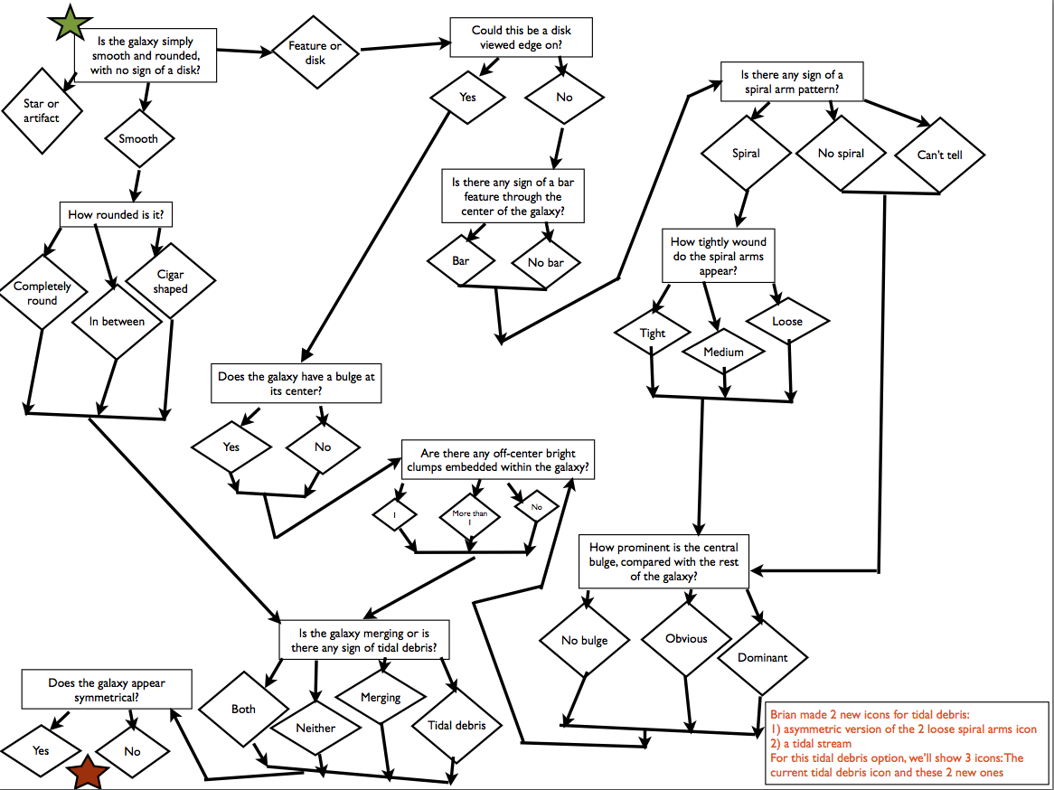Posted May 2, 2014 2:16 PM