What bias does the varying fraction of Eos - in the QS catalog - introduce?
-
 by
JeanTate
by
JeanTate
Consider AGS00001uz:
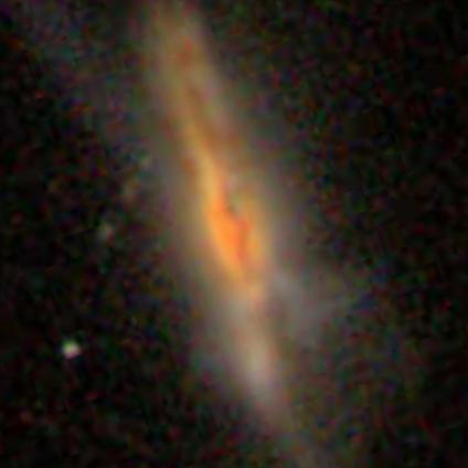
It's classified as an Eos ("Could this be a disk viewed edge-on?" "Yes"), has a redshift of 0.016, and is in the Composite part of a BPT diagram. Which means that the two ratios of emission line fluxes are best accounted for (explained by) both an AGN and star-forming regions in the part of the galaxy sampled by the light entering the spectroscopic fiber.
Compare this QS object with AGS000019r:
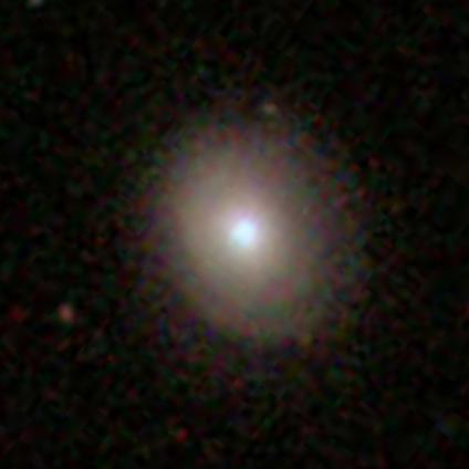
It's classified as completely round, has a redshift of 0.022, and is in the AGN part of a BPT diagram. Which means that the two ratios of emission line fluxes are best accounted for (explained) by an AGN in the part of the galaxy sampled by the light entering the spectroscopic fiber.
If the latter galaxy were viewed edge-on (assuming it is, in fact, a disk galaxy!), would we have pegged it as a Composite?
In other words, to what extent are our classifications biased by viewing galactic nuclei (with the SDSS spectroscope) through thousands or tens of thousands of parsecs of galactic disk?
One way to try to answer this is look at the distribution of 'BPT classification' by 'Eos or not'.
In this thread I'd like to present the results of some analyses I've done into this.
I began by excluding outliers: the ~100 QS objects I mentioned in the first post of page 2 of the What is needed to get a clean QS and a clean QC? thread (my write-up of those is a WIP) and QS objects with unknown stellar mass (log_mass = -1); 2813 objects remained.
Next I classified all these by 'BPT type' (details are in the BPT diagrams from the SDSS spectroscopic pipeline thread): AGN (1 in the table below), SF (2), Composite (3), low S/N AGN (4), low S/N SF (5), and Unclassifiable (6). Here is the distribution by Eos ("Could this be a disk viewed edge-on?" "Yes") or not (everything else):
      Eos    1   2   3   4   5   6
      Yes   11 129  50  12   0  16
      No   498 847 508 427  76 239
Yes, a chi-square test, of this as a contingency table, has a p of zero; the two distributions are rather different, statistically speaking.
But what if AGN, Composite, and low S/N AGN are combined (so we'd test for 'evidence of an AGN')? And SF and low S/N SF too? And the Unclassifiables are removed? Same result: the two distributions are rather different, statistically speaking.
I repeated the analysis, independently, on a subset of 1193 QS objects - mostly the bigger and closer ones - dividing them into 'Eos', 'maybe Eos', and 'not Eos' categories, by 'visual inspection' (I think that's the technical term!) of the DR10 images. Here are the results:
      Eos     1   2   3   4   5   6
      yes     6 173  34   4   0   4
      maybe  13 119  33   5   0  10
      no    147 325 150  89  10  71
Once again, statistically speaking (per chi-square contingency table tests), the distributions are different. No matter how you combine cells (sensibly!). The closest to similar is 'combined AGN' vs 'combined SF' for yes vs maybe (p=0.027).
So, among QS objects, the fraction of Eos with evidence of an AGN is far smaller than the corresponding fraction for non-Eos.
Why does this matter? Because the 'Eos fraction' is not constant, in the QS catalog, by redshift or stellar mass. For example, from page 2 of the Quench: Sample vs Control, what's the same, what's different thread ('Eos fraction' in the second plot is the fraction of Eos among 'Features of disk' objects; as a fraction of all objects within a particular redshift bin it is approximately the product of the values in the two plots):


That means that whatever analyses we do concerning the presence (or not) of AGN in 'post-quenched galaxies', we need to be sure to address bias introduced by viewing angle (at least for disk galaxies)1.
Of course, with increasing redshift an Eos will become more difficult to classify as an Eos (cet. par.), so maybe the difference in distribution of BPT types is itself more apparent than real? Good question. I checked that out too, and the answer is ... (stay tuned!)
1 There's an important assumption here (maybe more than one), one that needs to be checked out; what?
Posted
-
by
JeanTate
in response to JeanTate's comment.
There's an important assumption here (maybe more than one), one that needs to be checked out; what?
One is: not all galaxies are spirals (have disks).
Repeating the analyses with the subset(s) of No (no) that is 'has features or disk' makes no difference to the conclusions: the 'BPT type' distribution for Eos is significantly different (statistically, chi-square test on contingency tables) than that for non-Eos 'disk galaxies' (per zooite's classifications).
Here, for example, is what the first table looks like, with 'No' being restricted to objects zooites classified as 'has features or disk' (and 'not Eos'!):
      Eos    1   2   3   4   5   6
      Yes   11 129  50  12   0  16
      No   194 575 274 136  16  97
Next: what if only a narrow range of redshift or log_mass is selected?
UPDATE: As I had earlier found some evidence (it's on page 2) for objects classified as 'Cigar shaped' being (highly inclined) disk galaxies, I also repeated the distribution analysis assuming 'Cigar shaped' QS objects are disk galaxies but not Eos1. Same result.
1 Some undoubtedly are, in fact, Eos. I plan to look into this in more detail later.
Posted
-
by
JeanTate
I just realized: the analysis I just reported could be repeated for the QC objects, using Tools.
While it was important to remove the outliers for QS objects, it may be less so for QC ones. Why? For starters, there are only five (?) 'log_mass = -1' QC objects, vs ~110 in QS. Identifying the different 'BPT types' with Tools will certainly be tedious (and error-prone), but is certainly do-able.
Would anyone else like to give it a try?
Posted
-
by
JeanTate
Rank all 2813 QS objects by redshift; divide them into 24 bins of equal size (number). From the zooite classifications, work out the 'Eos fraction' in each bin (i.e. number of Eos in bin x divided by number of objects in bin x); from analysis of the emission lines, work out what 'BPT type' each is - AGN, SF, Composite, etc. For each bin, calculate the 'pure AGN fraction' and the 'at least some evidence for AGN fraction'. Plot them.
For example, there are 26 Eos in the first redshift bin, 12 'pure AGNs', and 18 objects for which there is some evidence - in the spectra - for an AGN. So the Eos fraction for redshift bin #1 is 0.22 (26/117), the 'pure AGN' fraction 0.10 (12/117), and the 'other AGN' fraction 0.15 (18/117).
Here's the plot, with linear trend lines added:

The redshift bins with high AGN fractions - of either kind - have close to zero Eos, and vice versa ... but the relationship is not very tight.
Now, rank the 2813 QS objects by petro_r50, divide them into ... you get the idea; repeat the above, but this time using apparent size. Here's the result:

The same general trends hold, but with two key differences:
- for the 'evidence for AGN' trend, the scatter is considerably greater
- the 'pure AGN' trend is much closer to two lines than one: for Eos fractions > ~6%, the line is very steep; for < ~6%, it's almost flat.
What if we create 24 log_mass bins; what do the Eos fraction vs AGN fraction plots look like? Like this:

A mess.
Having gone to the trouble of creating three sets of bins, I was curious to know what the stellar-mass (as estimated by the log_mass parameter) - redshift relationship looks like, viewed from the perspective of three different binnings.
Recall, back in the beginning of November, trouille posted this plot (it's on page 4 of the Mass Dependent Merger Fraction (Control vs Post-quenched Sample) thread):

Here's a presentation of a subset of that data, from three different perspectives (the blue, green, and orange/red in the two different plots have nothing to do with one another):

The two points with error bars show the approximate 68% variation, per this MPA webpage (the log_mass values in the QS catalog come from the "MPA-JHU DR7 release of spectrum measurements", I think); the one at the right is at log_mass =10.5, which is the mean for the 2813 objects. That's not a coincidence; to try to get a handle on Eos and AGN, I made a 'constant mass' selection centered on 10.5. A horizontal slice 0.3 dex thick in fact. Stay tuned.
Posted
-
by
JeanTate
Oh, I forgot one plot:

That's the Eos fraction for each of the 24 log_mass bins; there's certainly some scatter, but the trend is pretty clear: Eos fraction decreases with increasing stellar mass. But so it also does with redshift; are there two effects here, or only one? And is this only an apparent effect (or two), due solely to how QS objects were selected in the first place?
Posted
-
by
JeanTate
in response to JeanTate's comment.
For example, there are 26 Eos in the first redshift bin, 12 'pure AGNs', and 18 objects for which there is some evidence - in the spectra - for an AGN. So the Eos fraction for redshift bin #1 is 0.22 (26/117), the 'pure AGN' fraction 0.10 (12/117), and the 'other AGN' fraction 0.15 (18/117).
To clarify: the 12 'pure AGN' are a subset of the 18; however, the 26 Eos are unrelated. In light of what I wrote earlier, you'd expect only a handful of the 26 Eos to be among the 18 (and perhaps only one among the 12)1. Turns out there are three (and one):
Left to right: AGS00001ne (the 'pure AGN', z=0.015), AGS00000i4 (a 'low S/N AGN', z=0.023), and AGS00001uz (a Composite, z=0.016).
- the 'pure AGN' trend is much closer to two lines than one: for Eos
fractions > ~6%, the line is very steep; for < ~6%, it's almost
flat.
Here's a plot that makes this much clearer (the diamonds are the first eight - of 24 - 'petro_r50' bins, the crosses the other 16):

1 formally, 8.7 and 1.3 respectively. Of course, the 'sample size' is small (and most definitely not selected randomly), so 'expected values' come with huge caveats!
Posted
- the 'pure AGN' trend is much closer to two lines than one: for Eos
-
by
JeanTate
Time to look at the '10.5±0.15' log_mass subset. As I mentioned above, this is centered on the QS sample mean, and loosely one can think of all 701 objects as having 'the same stellar mass'. Not strictly true of course - and as some point I plan to look into how reliable the MPA-JHU DR7 estimates are likely to be, given how QS objects were selected - but the stellar masses are likely to be the same, within a factor of 2 or so.
Here's a pretty amazing factoid: this 'fixed mass' subset comprises almost a quarter (701/2813) of the entire QS sample! 😮
For my first set of analyses, I repeated the redshift-binning, to create 12 equal-sized (by number) redshift bins; the bin means range from 0.05 to 0.17; the first and last bins are quite wide (as you'd expect), but the other ten are only ~0.01 wide (i.e. the minimum redshift in any of these bins is only ~0.01 less than the maximum redshift).
As above, I looked at 'bin fractions'; for example, the fraction of objects in each bin that are Eos, say, or have 'pure AGN' emission line spectra. As an intro, a small surprise: combine the 'Composite' and 'low-S/N AGN' BPT types (or classes), and you find these are roughly constant, as a fraction, across redshift-bin, for the first eight bins (they range from 0.29 to 0.36), then rise rather smoothly for the last four (0.40, 0.47, 0.47, and 0.49, respectively). Why?
(to be continued)
Posted
-
by
JeanTate
in response to JeanTate's comment.
Here are the trends, by redshift, for the 'pure AGN' fraction (blue) and 'at least some evidence of AGN' fraction (orange), in the '10.5±0.15' log_mass subset:

Variation in the first eight bins is driven mainly by changes in the 'pure AGN' fraction, though they may be statistically insignificant (except for the first bin); there does seem to be a significant change starting around z=0.12. Main point, however: more than half the '10.5±0.15' QS objects have evidence of an AGN.

The Eos fraction declines with increasing redshift, becoming indistinguishable from zero at around z=0.11. Is this purely a "you can't tell if they're '10.5±0.15' Eos or not, beyond z~0.1" effect? Possibly:

"Features or disk" includes Eos; yes, that (fixed mass) fraction declines with increasing redshift too, but it seems less smooth (though that may be just statistical noise). Just looking at the fractions themselves, from z~0.09 on, the majority of 'evidence of AGN' objects are 'smooth'.
Assume 'Cigar-shaped' QS objects, in the '10.5±0.15' subset, are all disk galaxies; add them to the 'features or disk' fraction:

Same general trend. Now what?
Posted
-
by
JeanTate
in response to JeanTate's comment.
Now what?
Well, back to the OP!
Of course, with increasing redshift an Eos will become more difficult to classify as an Eos (cet. par.), so maybe the difference in distribution of BPT types is itself more apparent than real? Good question. I checked that out too, and the answer is ... (stay tuned!)
And the second post (bold added):
Next: what if only a narrow range of redshift or log_mass is selected?
Of the 59 Eos in the "10.5±0.15" log_mass subset, 23 show 'evidence of AGN' (and just two 'pure AGN'1). Is this distribution, as a 2x2 contingency table, consistent with that of the global distribution, involving 218 Eos (73 of which show 'evidence of AGN')? Yes; with 1 dof and a chi-square value of 0.62, p is 0.431. The expected number of 'pure AGN' Eos is ~3.5; while 2 seems consistent with this, the numbers are far too small to perform any meaningful statistical analysis2.
What about the non-Eos in this subset? For both 'pure AGN' and 'evidence of AGN', the answer is 'no, but barely'. For the former, a 2x2 contingency table gives a chi-square value of 3.75 (p=0.054, 1 dof); for the latter, 3.55 (p=0.059, 1 dof). In both, the expected number of pure AGN (128) and 'evidence for AGN' (360) is less than the actual (145 and 381, respectively).
But with the large range of redshifts, and the strong correlation with redshift for the Eos fraction, is the consistency physically meaningful (other than suggesting that there's a strong 'redshift bias' at work)? And for AGN fractions (both kinds), does the marginal significance (compared with the global distributions) point to a real mass-dependent effect? Or do the (mild) variations with redshift hint at heterogeneous populations (for example)?
1 You're itching to know what they look like, right? For example, are they starkly mono-color (yellow-ish white), like AGS00001ne? Behold! AGS00000iu (left, z=0.080) and AGS000013n (right, z=0.039):
I love surprises, don't you? 😉
2 As far as I know. If you think there is - possibly - such an analysis, please say so!
Posted
-
by
JeanTate
in response to JeanTate's comment.
I love surprises, don't you? 😉
AGS000013n with its "Warnings: NEGATIVE_EMISSION" came as complete surprise to me; I didn't even know what it looked like until the moment I posted the image link. 😮
Earlier, referring to ''Cigar shaped' QS objects', I wrote:
Some undoubtedly are, in fact, Eos. I plan to look into this in more detail later.
Butterfly me got to wondering, of the 60 'Cigar shaped' QS objects in the '10.5±0.15' log_mass subset, how many are 'pure AGN' (in terms of their BPT type)? And are they, in fact, Eos?
Well, the answer to the former question is "four"; the answer to the latter? You be the judge:
Left to right:
- AGS0000095 z=0.075
- AGS00001kv z=0.054
- AGS0000286 z=0.083
- AGS00002ay z=0.068
Posted
-
by
JeanTate
One last post before taking a 'constant redshift' cut. Mergers.
Taking 'Merging', 'Disturbed', 'Tidal debris', and 'Both' as 'merging' - and so 'Neither' as 'not' - the 'merging' fraction for the '10.5±0.15' log_mass subset is 15.6%. By redshift bin, it jumps around a fair bit, from 7% to 22%, starting and ending on a high:

Of the ~15% of QS objects (in this log_mass sample) which show signs of merger activity, none are Eos in the four redshift bins with the greatest redshifts; not really surprising as there are almost zero Eos in these bins. Much the same for the middle four redshift bins. For the first four (lowest redshift) bins, about a quarter of the merging QS objects are Eos.
What about nuclear activity; how many QS objects with 'pure AGN' spectra are also merging? And are there any 'merging' objects for which there is no evidence of AGN activity?

Overall, about a quarter of the 'merging' objects have 'pure AGN' nuclei, and about a fifth of those with such nuclei show signs of merger activity. However, there are wide variations: in one redshift bin there are no 'merging' objects with 'pure AGN' nuclei; in another, almost all have such nuclei.

Only a minority of QS objects which have 'evidence of an AGN' are 'merging' (~10% to ~25%), but a majority of the 'merging' objects have 'evidence of an AGN' (in one bin, all of them). The way the orange diamonds jump around in apparent synch with the black ones - much more so than either the blue or green ones do - tells us ... what?
Posted
-
by
JeanTate
What about the colors of the QS '10.5±0.15' log_mass subset? Not the apparent colors, but the absolute ones? The v4 QS catalog has five fields - x_absmag, where x={u,g,r,i,z} - which we can use to get answers. As there are few Eos in the highest eight bins, I combined them into two, #5-#7, and #8-#12. Here are the (absolute) u-r and g-i colors (the latter have been shifted up 1.05 mag, to highlight differences):

No particularly obvious trends, except a possible tendency for Eos to become slightly bluer - in both colors - at higher redshifts.
When the full '10.5±0.15' dataset is plotted, just such a trend is clear:

The g-i colors are more or less constant in the first four bins, then become bluer, monotonically. For u-r it's not so obvious what's going on, except that whatever 'bluing' there is, it's far weaker than that for g-i.
A plot of the absolute mags themselves is highly revealing (NOTE: y-axis is reversed; brighter at the top; pale green crosses are the Eos, only u, r, and z plotted):

Two things leap out at me (but YMMV, of course): either the objects are heterogeneous or it's volume limited to about bin #4 or #5; and the higher redshift objects are bluer, in all colors1.
Are the Eos significantly different (from the general '10.5±0.15' population), in terms of absolute mag or color? Stay tuned!
1 The r-i trend is particularly strong
Posted
-
 by
trouille
scientist, moderator, admin
by
trouille
scientist, moderator, admin
I'm very interested to see how this analysis plays out with the more restricted Quench sample (see this post for details). If you can redo the analysis, could you include error bars?
You can use the approach described here, with error = numerator/denominator:
numerator = square_root (# of sources in bin with given characteristic)
denominator = total # of sources in bin
Posted
-
by
JeanTate
in response to trouille's comment.
Fairly easy to repeat this with a QS subset, which I'll do.
Could you clarify please, concerning 'error bars'? You're referring to plots in which the y-axis is 'fraction' (or similar), right?
I mean, if the y-axis is 'absolute magnitude' (or similar), the error bars should be derived from the stated errors of the SDSS modelmags, the errors introduced by the k-correction, etc, shouldn't they?
Posted
-
by
JeanTate
In this post I report on some of the "Eos" distributions; not a subset selected by (narrow range of) redshift, but rather 'the 778' per Laura's post:
- 0.02 < redshift < 0.08 AND
- z_absmag < -19.5 AND
- log_mass != -1
For differences between the 778 QS objects and their control counterparts, check out Characterizing 'the 778': how do the QS objects differ from the matched/paired QC ones?
In marked contrast to the results in the first two posts of this thread, the distributions of 'BPT type' by 'Eos or not', among both QS and QC objects among 'the 778', are not statistically significantly different (in general).
For example, for the three main 'BPT types' - 'AGN (1), 'SF' (2), and 'Composite (3), here is the QS distribution, comparing 'Eos' with 'rfod' (rest of 'Features or Disk'), followed by the QC distribution1:
QS:   1  2  3 QC: 1   2  3
Eos   7 68 25     4  33 17
rfod 18 72 32    13 109 24
The QS distribution is not statistically significant (chi-squared 3.67, 1 dof, p=0.16), and the QC similarly (or perhaps marginally; chi-squares is 5.47, 1 dof, p=0.065).
There are some curious differences between the QS and QC distributions ... but some of the cells have rather few members, so perhaps the statistical significance isn't what it might otherwise appear to be. For example: combining 'AGN', 'Composite', and 'weak AGN' into 'some evidence for AGN' ('eAGN'), and combining 'SF' and 'weak SF' into 'some evidence for SF' ('eSF'), with the rest - 'unclassifiable' - being 'else', Here are two pairs of distributions ('nEos' means 'everything except Eos'):
QS: eAGN eSF else QC: eAGN eSF else
Eos  36   69   2       29   42   3
rfod 56   74  13       49  141   3
A 3x2 contingency table chi-square(d) test gives (2 dof): 7.1, p=0.029 (QS) vs 7.05, p=0.029 (QC)
A 2x2 one (eAGN and eSF only), with 1 dof, 1.88, p=0.17 (QS) vs 5.59, p=0.018 (QC)QS: eAGN eSF else QC: eAGN eSF else Eos 36 69 2 29 42 3 nEos 267 366 38 181 480 43A 3x2 contingency table chi-square(d) test gives (2 dof): 5.11, p=0.078 (QS) vs 6.29, p=0.043 (QC)
A 2x2 one (eAGN and eSF only), with 1 dof, 2.32, p=0.128 (QS) vs 5.68, p=0.017 (QC)1 Yes, there are relatively more Eos among the QS objects; see Characterizing 'the 778': how do the QS objects differ from the matched/paired QC ones? for details.
Posted
-
by
JeanTate
in response to trouille's comment.
First attempt:
- 'the 778', all of them
- 12 'equal-sized' redshift bins, based on QS redshift distribution
- the fraction of Eos by redshift bin
- with error bars (per Laura's post)
- for both QS and (matched) QC objects

An example, the first redshift bin:
- 65 QS objects (blue), 65 QC ones (orange)
- mean QS redshift is 0.02874, mean 'QC redshift' is the same1
- 13 QS Eos in this bin, and 3 QC ones
- QS ±error bar is thus 0.055 - SQRT(13)/65 - and QC one 0.027 - SQRT(3)/65
Is this correct?
Why this formula for the error bars?
In any case, the QS/QC redshift distribution of Eos is ~the same from ~0.045, but at lower redshifts there are more QS Eos (relatively).
1 I don't think this is the right way to do this; however, I expect the difference - using proper mean QC redshift bins - will be small; I'll do that analysis later
Posted
-
by
JeanTate
in response to JeanTate's comment.
however, I expect the difference - using proper mean QC redshift bins - will be small; I'll do that analysis later
Here it is:

In at least one respect the difference is indeed small: for only the first two (and perhaps the last) redshift bin is there any apparent different of any note:
- among the first ~130 or so objects (two redshift bins), the QC Eos fraction is (much) less than that of the corresponding QS one; is this significant? stay tuned!
- the difference for the highest redshift bin is ... strange; however, I think it's largely an artifact of how the QC objects were selected, rather than a "that's the way it is, physically, among the relevant galaxies" (or something similar).
Posted
-
by
JeanTate
OK, so the plot in the last post treats the QC objects as independent (from the QS ones), which they are (the 778 galaxies have nothing to do with one another!), but also are not (each QS object has a QC counterpart, or match).
The way to preserve this independent-yet-not character is to keep the QC objects' redshifts, but analyze them using the QS objects redshift bins.
Perhaps an example or two will help.
Consider AGS00002br ("2br" for short): it's a QC object, paired with/the counterpart to the QS object AGS000000d (''00d" for short). 00d's redshift is 0.022, putting it into the QS redshift bin #1; 2br's redshift is 0.015, which is also in bin #1.
What about AGS00001hr ("1hr")? It's a QS object, with redshift 0.046, putting it into bin #3. Its counterpart is AGS00003t5 ("3t5"), which has a redshift of 0.027. If 3t5 were a QS object, it'd go into bin #1; however, as it's paired with 1hr, it goes into bin #1.
Here's the revised plot:

Pretty much the same conclusion: Eos fractions are markedly different up to a redshift of ~0.04; beyond that, apparently very similar.
(actually it's not quite right; the denominators for the error bars are no longer 65 - the number of QS objects in each redshift bin - but something else; I'll re-do this and repost).Um, I must not have had enough coffee ... the number of QC objects in bin #1 (to take just one example) is the same as the number of QS objects in that bin, because QC objects are paired with QS ones! What the plot in this post is showing - albeit not very clearly - is that there is a systematic difference between the distribution of the QS redshifts and the QC ones (the plot in the last post also shows that too, also not very clearly). Which is indeed true:

The x-axis is the redshift of QS objects minus that of their QC counterparts; the y-axis is the same, but for log_mass (for 'the 778'). There are more points to the left of dz=0 than to the right; the mean of the distribution is -0.0031. For dlm it's not so obvious that there's an imbalance; the mean is 0.0013. It's easier to see this if the 'width'1 of the distributions is forced to be equal, by dividing each point by the standard deviation of their respective distributions. The mean of the 'semi-normalized'1 dz distribution is -0.25, and that of the corresponding dlm one 0.05.
A CDF (cumulative distribution frequency) plot, of the two semi-normalized distributions, brings this out very clearly:

The yellow is the CDF of a normal distribution (Gaussian) with mean = 0 and standard deviation of 1.
But does this matter, in terms of an analysis of 'the 778'? I don't think so.
1 what's the technical term for these?
Posted
-
by
JeanTate
Turning to how the Eos fraction varies with stellar mass.
Back on page 1, for the whole QS catalog (sans a small number of outliers), I posted this plot:
That's the Eos fraction for each of the 24 log_mass bins; there's certainly some scatter, but the trend is pretty clear: Eos fraction decreases with increasing stellar mass. But so it also does with redshift; are there two effects here, or only one? And is this only an apparent effect (or two), due solely to how QS objects were selected in the first place?
Here's the equivalent for 'the 778', with error bars, and adding QC objects (and switching the axes):

With the possible exception of a small range around 10.1 (log_mass), the QS and QC fractions are 'the same'. And Eos fraction increases with stellar mass .... (pause) .... (waiting for the penny to drop) ...
Yep, the exact opposite trend from the one that seems clear in the full sample! 😮
To make this obvious, here's the full sample data plotted on top of 'the 778':

Don't you just love astronomy? Always full of surprises! 😄
Posted