What do BPT diagrams look like, if you select for fiber covering fraction?
-
 by
JeanTate
by
JeanTate
I'll add the background - brief description, links to other posts/threads here - later.
For now, three quick plots: starting with the QS (v4) objects in mlpeck's CasJob group (N=2793), and cutting on emission_line_flux > 0 (for H-alpha, H-beta, [OIII]5007, and [NII]6584), and S/N > 3 (same emission lines) (N=2025), I created three groups:
- all five SDSS bands have fiber covering fractions > 20% (per Kewley et al 2005) (N=1247);
- all bands with fiber covering fractions < 20% (N=319); and
- the rest (at least one band with a fiber covering fraction > 20%, and at least one band < 20%) (N=459)
Here are the BPT diagrams for each, with the axes ranges fixed (and the same for all three):


While the N's are quite different - so visually the plots are hard to compare - it seems that covering fraction is important. I'll do some further analyses later, and have a go at estimating whether the differences are, in fact, significant.
Of course, QS objects with large covering fractions have - on average - higher redshifts (and log_masses) than those with small ones. Too, several of those with small covering fractions are not centered on galactic nuclei (so can't end up in the 'AGN' part of the BPT diagram). So I'll also have a go at estimating if any covering fraction differences are due, in fact, to log_mass differences.
One other thing occurred to me: how do 'whole galaxy' colors differ from 'fiber colors'? Or, for a fixed fiber covering fraction, what is the range of color difference? This color difference is likely a proxy for how different the bulge color is from that of the disk (and also how big the bulge is, compared to the disk).
What do you think?
Posted
-
by
JeanTate
OK, do I win the 'lead balloon' award? A day later, and not a single response. 😦
Anyway, I wasn't able to find any papers on aperture effects and BPT diagrams (re SDSS spectra), so I asked that question in the CosmoQuest forum: How does the BPT position of an object change, as the covering fraction varies? And I got some answers (read the thread for details).
Bottom line? For such rare and unusual objects as post-quench galaxies, extrapolating from spectra which sample < ~20% of the galaxies' light is fraughtfraught.
So I propose that we exclude all such objects, forthwith.
There's a corollary: we should revisit the control objects, and for the matched controls for QS galaxies which survive my proposed 'fiber covering' cut, make sure they all have fiber covering fractions > 20%. If not, back to the selection drawing board.
Radical? Yes. Good science? I think so.
But you may well disagree. As a fellow zooite - and possible co-author - would you please say why? And if you disagree, would you please say how you think we can control for the unknown (and, as today, unknowable?) biases introduced by assuming small-aperture-spectra can be reliably extrapolated to 'whole galaxy' parameter values?
Posted
-
 by
mlpeck
by
mlpeck
I read it, I just have no idea how to respond.
You propose to remove, by your count, nearly 60% of the sample? Based on an 8 year old paper and a couple of responses on a web forum?
I think you have some work to do to make a convincing case. I'd suggest, for a start, taking a look at color gradients as a function of covering fraction. I'd also suggest reviewing some of the relatively small body of literature involving IFU (or otherwise spatially resolved) spectroscopy.
Posted
-
 by
jules
moderator
by
jules
moderator
I'm here and also have no idea how to respond. I really don't know how big a deal this is but it's certainly worth asking. I think we need a scientist to comment.
Posted
-
 by
zutopian
by
zutopian
Interesting topic. I follow the discussions in Talk and Cosmoquest.
Posted
-
by
ChrisMolloy
in response to JeanTate's comment.
I don't know how to respond to this. But have followed with interest. Intrigued as to how this will be resolved.
Posted
-
by
JeanTate
Thanks everyone. Heartening to see all the zooites currently active in Quench here in this thread! 😃
I began this thread with "I'll add the background - brief description, links to other posts/threads here - later." Big mistake; sorry 😦
In this post I'll start giving the background etc; please bear with me, it may take more than one post (I'll already lost one draft; I must have clicked something wrong somewhere ...).
Let me start with Kewley et al. (2005) - "APERTURE EFFECTS ON STAR FORMATION RATE, METALLICITY AND REDDENING" - which jtmendel (moderator, scientist) introduced us to (4th post in this thread). Here's the abstract (copy/pasting is not perfect):
We use 101 galaxies selected from the Nearby Field Galaxy Survey (NFGS) to investigate the effect
of aperture size on the star formation rate, metallicity and reddening determinations for galaxies. Our
sample includes galaxies of all Hubble types except ellipticals with global SFRs ranging from 0.01 to
100 M⊙yr−1, metallicities between 7.9 <log(O/H)+12 <9.0, and reddening between 0 <A(V ) ❤️.3.
We compare the star formation rate, metallicity and reddening derived from nuclear spectra to those
derived from integrated spectra. For apertures capturing < 20% of the B26 light, the differences
between nuclear and global metallicity, extinction and star formation rate are substantial. Latetype
spiral galaxies show the largest systematic difference of ∼ 0.14 dex in the sense that nuclear
metallicities are greater than the global metallicities. Sdm, Im, and Peculiar types have the largest
scatter in nuclear/integrated metallicities, indicating a large range in metallicity gradients for these
galaxy types or clumpy metallicity distributions. We find little evidence for systematic differences
between nuclear and global extinction estimates for any galaxy type. However, there is significant
scatter between the nuclear and integrated extinction estimates for nuclear apertures containing < 20%
of the B26 flux. We calculate an ‘expected’ star formation rate using our nuclear spectra and apply
the commonly-used aperture correction method. The expected star formation rate overestimates the
global value for early type spirals, with large scatter for all Hubble types, particularly late types. The
differences between the expected and global star formation rates probably result from the assumption
that the distributions of the emission-line gas and the continuum are identical. The largest scatter
(error) in the estimated SFR occurs when the aperture captures < 20% of the B26 emission. We
discuss the implications of these results for metallicity-luminosity relations and star-formation history
studies based on fiber spectra. To reduce systematic and random errors from aperture effects, we
recommend selecting samples with fibers that capture > 20% of the galaxy light. For the Sloan
Digital Sky Survey and the 2dFGRS, redshifts z > 0.04 and z > 0.06 are required, respectively, to
ensure a covering fraction > 20% for galaxy sizes similar to the average size, type, and luminosity
observed in our sample. Higher-luminosity samples and samples containing many late-type galaxies
require a larger minimum redshift to ensure that > 20% of the galaxy light is enclosed by the fiber.That paper has been cited by 127 others, according to ADS. I tried to find, and read, all those which are relevant to us. One in particular clearly is: Gerssen et al (2012) "Beyond the fibre: resolved properties of Sloan Digital Sky Survey galaxies" (thank you, matt.o):
We have used the VIMOS integral field spectrograph to map the emission line
properties in a sample of 24 star forming galaxies selected from the SDSS database. In
this data paper we present and describe the sample, and explore some basic properties
of SDSS galaxies with resolved emission line fields. We fit the H α+[NII] emission
lines in each spectrum to derive maps of continuum, Hα flux, velocity and velocity
dispersion. The H α, Hβ , [NII] and [OIII] emission lines are also fit in summed spectra
for circular annuli of increasing radius. A simple mass model is used to estimate
dynamical mass within 10 kpc, which compared to estimates of stellar mass shows
that between 10 and 100% of total mass is in stars. We present plots showing the
radial behaviour of EW[Hα ], u-i colour and emission line ratios. Although EW[H α]
and u-i colour trace current or recent star formation, the radial profiles are often quite
different. Whilst line ratios do vary with annular radius, radial gradients in galaxies
with central line ratios typical of AGN or LINERS are mild, with a hard component of
ionization required out to large radii.We use our VIMOS maps to quantify the fraction
of Hα emission contained within the SDSS fibre, taking the ratio of total Hα flux to
that of a simulated SDSS fibre. A comparison of the flux ratios to colour-based SDSS
extrapolations shows a 175% dispersion in the ratio of estimated to actual corrections
in normal star forming galaxies, with larger errors in galaxies containing AGN. We
find a strong correlation between indicators of nuclear activity: galaxies with AGN-like
line ratios and/or radio emission frequently show enhanced dispersion peaks in their
cores, requiring non-thermal sources of heating. Altogether, about half of the galaxies
in our sample show no evidence for nuclear activity or non-thermal heating. The fully
reduced data cubes and the maps with the line fits results are available as FITS files
from the authors.And I've found at least two others which seem particularly pertinent (I'll post details of those later).
Take-away: yes, I've been doing exactly what you suggest, mlpeck, and so far everything I've found is consistent with 'extrapolating from SDSS spectra, with covering fractions of < 20%, to estimate global (galaxy) properties is unreliable'.
Lastly, for this post: "remove, by your count, nearly 60% of the sample?" No. "covering fraction" is measured by integrated flux (Kewley et al.'s "apertures capturing < 20% of the B26 light"). For the 2025 QS objects I used to produce the BPT diagrams, that's ~40% (319+459).
Posted
-
by
JeanTate
Three more papers directly relevant to this thread (I won't post abstracts for these): Moustakas et al (2006), Iglesias-Páramo et al (2013), and Pracy et al, (2013). The latter two present observational results consistent with 'extrapolating from SDSS spectra, with covering fractions of < 20% [or similar], to estimate global (galaxy) properties is unreliable'; the first has a Table (two actually) from which integrated vs nuclear emission line ratios can be derived, but I have not yet downloaded the data, much less analyzed it.
I'd like to quote from the conclusion in [Iglesias-Páramo et al (2013): "We finally add that this paper presents only the tip of the iceberg. Aperture effects are widely mentioned but rarely understood. Their influence can seriously affect scientific results through systematic errors (Bland-Hawthorn et al. 2011)."
Posted
-
by
JeanTate
More background: the Redshift and size cuts: Proposal and discussion thread - which I already linked to - is good (as background!)
In the OP, I wrote: "the QS (v4) objects in mlpeck's CasJob group (N=2793)". Sadly, I cannot now find the thread/post which describes this group 😦 I used it ("quenchdb" is its name) to obtain the fiberMags and cModelMags (five each, for each; one for each band), as well as their respective errors.
Why 2793, and not ~3002? Because mlpeck matched the plate and fiber ID, from the QS catalog, and for ~205 QS objects it's not easy to find the corresponding fiberMag (etc). How come? Because for those objects, the spectrum (SpecObjID) in the QS catalog is not primary 😮 What does that mean? That for these there is another spectrum - from a different plate/mjd/fiber - which is primary.
That leaves me in a bit of a quandary, for these: their status - as QS objects - derives from an analysis of what are now not primary spectra. Yes, I could go ahead and get the fiberMags and cModelMags for these, and use that data in any analyses. However, how to address the possibility that, had the (now) primary spectra been used, at least some of these objects would not have been selected (as post-quench galaxies)?
What do you think?
Posted
-
by
JeanTate
mlpeck: "I'd suggest, for a start, taking a look at color gradients as a function of covering fraction." Yes, I fully agree, and had intended to do just that anyway.
Here's a rough-and-ready first look:

The QS objects are the same as those used in the BPT diagrams; the black lines are equality; the colored lines linear trend lines.
These plots don't really show color gradients directly (I'll do that next, by plotting 'integrated color of that part of the galaxy that's outside the fiber footprint' instead of 'model (integrated) color'). Also, there are outliers - beyond the axes ranges - that affect the trend lines (yes, the orange line is surely too good to be true!). I'll also add the QS objects not in the BPT diagram, and think of a way to make plots showing trends with covering fraction.
But, quick check: with the caveats above, does any zooite think the covering fraction is irrelevant, in terms of this project?
Posted
-
by
mlpeck
In the OP, I wrote: "the QS (v4) objects in mlpeck's CasJob group
(N=2793)". Sadly, I cannot now find the thread/post which describes
this group 😦 I used it ("quenchdb" is its name) to obtain the
fiberMags and cModelMags (five each, for each; one for each band), as
well as their respective errors.Why 2793, and not ~3002? Because mlpeck matched the plate and fiber
ID, from the QS catalog, and for ~205 QS objects it's not easy to find
the corresponding fiberMag (etc). How come? Because for those objects,
the spectrum (SpecObjID) in the QS catalog is not primary 😮 What does
that mean? That for these there is another spectrum - from a different
plate/mjd/fiber - which is primary.I don't understand how you got this sample size. I only have 17 objects with missing photometry in my version of the data table, that is there are 2,983 with SDSS pipeline photometry (I have removed 2 obvious contaminants from my personal data table, leaving 3,000 in the quench sample).
But, quick check: with the caveats above, does any zooite think the
covering fraction is irrelevant, in terms of this project?I'm just going to give a very quick response for now because I'm getting just a tiny bit frustrated that 3 1/2 months into the "analysis" phase of this project we're still discussing sampling issues, and just about everything of more interest has ground to a halt. This is something that the lead investigator really needs to exercise some leadership on, preferably two months ago.
Anyway, what I think is the scientifically correct thing to do is to publish the catalog pretty much as is, and consider various subsets of the data. The last time she checked in Laura suggested some redshift cuts that would give us an approximately volume limited sample for example.
Posted
-
by
JeanTate
in response to mlpeck's comment.
I don't understand how you got this sample size.
The key part of my CasJobs Query is (obviously, I have omitted most of it; this fragment is invalid as a standalone Query):
SELECT s.SpecObjID,
from mlpeck.mlpeck54.quenchdb s, SpecPhoto p
WHERE s.SpecObjID = p.SpecObjID
In other words, where the SpecObjIDs don't match, no object in mlpeck.mlpeck54.quenchdb can be selected.
Anyway, what I think is the scientifically correct thing to do is to publish the catalog pretty much as is, and consider various subsets of the data.
Despite what I wrote in the second post in this thread, I agree 😮
To the extent that whatever trends or results we find are compromised/influenced/need-to-be-caveated/etc by selection effects (or whatever they might be called) such as fiber covering fraction (a.k.a. aperture effects), we should discuss these in our paper (as Wong et al. did - "In our sample, the observed spectral properties may not be representative for approximately 5 per cent of our sample where the outer galaxy regions are much greater than 3 arcsec and appear to be bluer than the central region.")
Posted
-
by
JeanTate
Here are the above BPT diagrams, with the object classes noted by different colors (yes, in the second there are two "SFR" which are wrongly labeled; and the AGN/Composite and Composite/SFR boundaries may not be as clean as they could be).

A 3x3 contingency table gives a chi-square value of 295, with 4 dof that's a p of 0.000. In other words, the different distributions are statistically significant. Of course, as covering fraction is correlated with redshift, and as the QS sample has very significant Malmquist bias, redshift is correlated with log_mass. So I'll see if this huge fiber covering fraction bias/effect remains after 'correcting for' stellar mass.
             AGN Composite SFR
       lt20%  15      45   259
        ±20%  56     150   253
        >20% 447     372   428
Posted
-
by
JeanTate

Those plots are similar to the three above, except that the y-axis is the 'rest of object' (u-r) color, derived from working out the u and r band magnitudes of the 'rest of object' (because astronomical 'magnitude' is not a linear function of flux, you have to convert to flux, subtract 'fiber flux' from 'model object flux', then convert back to a magnitude).
I also removed outliers (see below). The three have the same axis ranges (x: [0.5, 4], y: [0, 5.5]); the colored lines are linear trend lines, and the black ones equality.
While there's a lot of scatter in the 'orange' plot (all covering fractions > 20%), there's no apparent systematic difference - the orange line is close to the black one, and they cross near the center.
There's less scatter in the blue plot, possibly because most of these objects are quite bright (e.g. mean r-band fiber mag is 16.3, cf 17.3 for the orange plot). However, there's a clear color gradient ('rest of object' is bluer than the part covered by the spectroscopic fiber, and the redder the object, the greater the gradient).
Green plot: the color gradients are more marked for objects which have at a covering fraction in at least one band > 20% and at least one < 20%. The scatter is also greater.
Outliers:
- 14 objects have a stated error in at least one (of 10) magnitudes > 2
- 15 objects have a covering fraction in at least one band that is >> 1 and/or wild colors (some quite crazy objects here!)
- 12 objects have a covering fraction in at least one band that is > 1; in effect, they are only ~3" in size.
(u-r) is not a good choice of color, to investigate aperture effects, even though it's a fave for separating blue cloud from red sequence galaxies in a CMD. Why? Because u-band errors (estimated u-band magnitudes) are greater than those in other bands (although z-band errors are sometimes greater), and many red objects have estimated u-band magnitudes that are pretty close to the sky (even if their formal errors are small). So next I'll take a look (g-i) colors, keeping covering fraction fixed (and using r-band covering fraction). Then I'll do what's surely a far more meaningful analysis: what aperture effect is there, when log_mass is held constant?
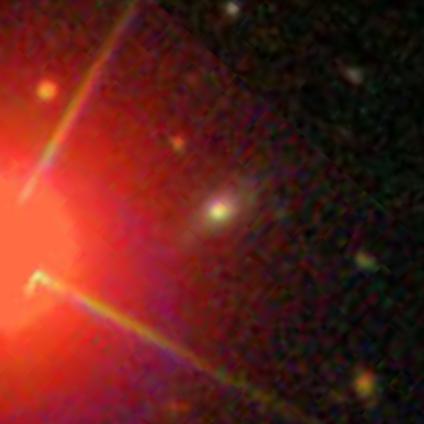
To close, one of the wildest of the 15: AGS00001b0:
This has an r-band covering fraction of 3.6, and a ModelMag of 20.3, which is obviously ridiculous ... until you realize that its PetroRad_r is ... wait for it ... 1.4" !!! In the QS catalog (v2), the r-band magnitude is 13.45, and petro_r50 22.7". Zoom out, add 'photometric objects' and 'spectroscopic objects', and you can see what's happening:
Posted
-
by
mlpeck
Salim et al. (2007) have a lengthy discussion of the aperture corrections that Brinchmann et al. (2004) performed to estimate star formation rates in SDSS galaxies -- see especially section 5. Their basic conclusion is that aperture corrected star formation rates for star forming galaxies are accurately estimated, while they are overestimated for other emission line classes.
The Brinchmann et al. models are the basis for the MPA-JHU pipeline measurements that we're using. Note also that stellar mass estimates are based on photometry only, so the quality issue with them relates to the accuracy of SDSS photometry pipeline size (and therefore model magnitude) estimates.
Posted
-
by
JeanTate
One of the things I find most interesting about astronomy is being surprised.

The blue points are the fiber (g-i) colors (x-axis) against the 'rest-of-object' (g-i) colors (y-axis); the blue line is the linear trend line; and the black line equality. Yes, there are points beyond all sides of the plot; I narrowed the range for an important reason.
Redward of (g-i) ~1, fiber colors tend to be redder than 'rest-of-object' colors; "discs are
redderbluer than bulges" might be nice narrative.But look at the orange diamonds, and the orange line which connects them!
I ranked the 2752 objects by r-band covering fraction, and then grouped them into ten bins, of 275±1 each. The ten orange diamonds are the mean fiber and 'rest-of-object' colors for each bin. The orange line joins the bins, in order. The bin means get redder - they 'move' up and to the right (bins 1 to 3), then get stuck, on the trend line (bins 4 to 6). Then comes the fascinating part: their 'rest-of-object' colors remain the same (the track is pretty much horizontal), but the fiber colors get bluer, monotonically! 😮
How come?
Now back to the boring 'aperture effects': the mean r-band covering fraction for bin 1 is 10.8%, and for bin 2 18.6%.
(more later)
Posted
-
by
JeanTate

The brownish-purple diamonds (and line) are the ten 'redshift' bins: I ranked the dataset by redshift and created ten equal-sized (275±1) bins. Lowest redshift bin is at the bottom left, and subsequent bins are redder than each previous bin, in both dimensions. This - qualitatively - is what I was expecting for the covering fractions.
The length of the line segment from bin 1 to bin 2 - in both orange and brown (for short) - and that from bin 9 to bin 10 in the brown one is no surprise; redshifts and covering fractions rise quickly from their minima, and redshifts rise rapidly again at the end of their range. That the brown line is below (redder) the black (equality) isn't at all surprising; galaxy outskirts are bluer than centers. At high redshift, covering fractions approach 100%.
That the orange line is below the brown one for the first three (maybe four) orange bins suggests that objects with smaller covering fractions are - on average - considerably bluer in their outskirts than their 'redshift average' (something to check). In turn, this seems to imply that - again on average - there are significant color gradients in objects with covering fractions <~25% (mean covering fraction in bin 3 is 23%; 27% in bin 4).
All a distraction from doing analyses with log_mass. 😦
Posted
-
by
JeanTate
in response to mlpeck's comment.
Thanks! 😃
There are quite a lot of AGN (including LINER) and composite objects in the QS catalog, as well as more than a handful of 'unclassified' (emission lines with S/N < 3, or no emission lines at all). The Salim et al. (2007) results suggest we'd be wise to treat aperture effects carefully - and differently - for each kind of object (based on position in a BPT diagram, or not in it at all).
The Brinchmann et al. models are the basis for the MPA-JHU pipeline measurements that we're using. Note also that stellar mass estimates are based on photometry only, so the quality issue with them relates to the accuracy of SDSS photometry pipeline size (and therefore model magnitude) estimates.
IIRC, quite some time ago we more-or-less agreed that quality problems with photometric pipeline derived parameters are different from those with spectroscopic pipeline derived ones. The former include (we have discussed some of these, but not all):
- unreliability near bright stars
- poorly estimated u-band magnitudes, especially formal errors that are unreasonably low (Salim et al. also mention this)
- blending and shredding (ditto) - a particular problem for the Eos (edge-on spirals), especially in the u-band.
We know, by the process of selection, that QS objects are very rare (~3k out of, what, ~900k MGS ones?). While they are surely composed of the same things other galaxies are - stars, gas, dust, AGNs - the detailed distributions (both spatially and population-wise) are surely at least somewhat different. Indeed, we know the stellar distributions (by spectral class) are very different; that's how they were selected (sorta)! True, it's a good first approximation to say we can apply the same stellar population models, dust models, etc to these objects - and that's all we can do, in the Quench Project! - but where we already know that a particular extrapolation (to do with covering fractions/aperture effects, in this thread) has known shortcomings/limitations, shouldn't we at least attempt to address it?
BTW (change of topic) I notice that "one of the wildest of the 15" (AGS00001b0) has two red squares ... I wonder if the other spectroscopic object in this Eos is also a QS object? What about other big Eos (where a QS object is a clump/photometric object well away from the nucleus)? Maybe a not-insignificant fraction of the QS objects are fairly ordinary SFRs viewed through a thick and highly uneven set of layers of dust in an Eos (and not post-quench objects at all)?
Posted
-
by
JeanTate
in response to mlpeck's comment.
How is covering fraction related to size, as measured by the Petro_r50 parameter in QS? Here's how:

That's all 2752 in previous plots, except that I've omitted three. Here are two of those, AGS00000s1 and AGS0000038:
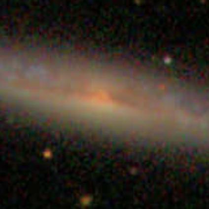
The first has a Petro_R50 of 22.5", making it the biggest - by far - among the 2752 (yes, the photometric pipeline can fail spectacularly near bright stars); the second, 0.71", making it no different from a star (yes, the photometric pipeline sometimes gets, um, overenthusiastic about breaking galaxies into tiny pieces; 'shredding' in Salim et al.'s words).
Posted
-
by
JeanTate
in response to mlpeck's comment.
Before what I think is pretty compelling evidence that there is a strong aperture effect that we need to seriously consider, a recap of the data.
Here's a plot just like the "QS objects: (g-i) colors" above, except that it has only 2651 QS objects ... the three Petro_R50 outliers I mentioned in my last post are gone, and those with "log_mass" with a value of -1. I've also created a similar plot, for (u-r) colors:

The orange lines are the tracks of covering fraction bins; brownish-purple redshift bins; and yellow log_mass bins (ten bins of equal size, in all cases). The (u-r) plot is messy; not only is the cloud of points far more extensive, but the lines jump around much more. Curiously, the orange line in the (u-r) plot doesn't double back.
With all lines buried deep inside clouds of points, can we see that they do, in fact, point to statistically significant aperture effects? Or are such effects simply a very subtle tendency for the cloud's centers to be slightly displaced from equality?
Stay tuned! 😃
Posted
-
by
JeanTate

As in previous plots of this kind, the black line is equality, and the blue the linear trend line. 530 QS objects are plotted, those with log_masses from 10.47 to 10.71 (log_mass bins 5 and 6); if I recall correctly, the formal uncertainties on log_mass are greater than 0.1 dex, so it's not a stretch to say that these objects all have the same stellar mass.
Also as above, the orange line and diamonds is the track of covering fraction bins. This time the lowest covering fraction objects are at the bottom right, and the track goes up then left. The number of objects in each covering fraction bin is not constant; these are 'full sample' bins; the number are - from bin 1 to bin 10 - 24 (%11.7%), 42 (18.7%), 42 (22.6%), 55 (26.1%), 45 (30%), 50 (33.1%), 66 (36.5%), 50 (41.4%), 73 (48.6%), and 83 (57.4%) (average covering fraction in brackets).
The purple triangles are the 24 in bin 1; blue triangles bin 2; and pink bin 10 (it would be very confusing to show all the others).
Yes, there are some blues among the pinks (3), and some pinks among the purples and blues (2), but the separation is almost total!
Case closed, wouldn't you say?
Posted
-
by
mlpeck
in response to JeanTate's comment.
Paper: Caught in the Act: Strong, Active Ram Pressure Stripping in Virgo Cluster Spiral NGC 4330 by Abramson et al. 2011. This is of course AGS00001b0 in the quench sample.
Posted
-
by
zutopian
in response to JeanTate's comment.
I guess, that your post is also somehow related to following case.:
There is still a known duplicate pair in the QS sample, though I had posted a reminder in the topics "Duplicates Summary" and "Outstanding questions".:Comment by mlpeck in the topic "Duplicates-Summary":
The QS-QS duplicate is at least slightly interesting. The spectra were recorded on two different plates with slightly different coordinates for the fibers, so two different regions of the same galaxy were sampled. The spectra are similar except that one is somewhat redder than the other. Only one of them is tagged as a "science primary" Here are the DR8 spectrum plots. The second one is the designated primary.
A long reply by Jean followed and in response following comment by mlpeck:
So, which to keep? My inclination would be to keep the one designated as the "science primary," but that's the one with the bad photometry at least in the DR7 database. It seems to have been corrected by DR9: http://skyserver.sdss3.org/dr9/en/tools/explore/obj.asp?sid=802910431264925696.
After my reminder post, Jean did following comment.:
AGS0000080 has a log_mass of 10.7796 and a redshift of 0.0474274; AGS00000j6's values are 11.0397, and 0.0478403, respectively. As you say, there will be QC counterparts to both these. The two log_mass values are not really all that close, so choosing one of the QS objects to exclude also means slightly changing the distribution of stellar masses (but, as it's just one object, that change will be very small indeed).
Posted
-
 by
trouille
scientist, moderator, admin
in response to zutopian's comment.
by
trouille
scientist, moderator, admin
in response to zutopian's comment.
Hi all, great catch on this duplicate source in the Quench sample. Interesting and something we need to remedy in our final clean sample. Is this source still in the final, restricted Quench sample (see this post for details)?
This duplicate reminds me of conversations happening now within the LSST community on whether to have each data release build on the last one (in terms of sharing ObjIDs) or start completely anew. LSST, like SDSS, is planning to start the ObjIDs new with each data release. And so we need to remember this experience in future studies to keep an eye out for duplicates like this one.
Posted
-
by
JeanTate
in response to trouille's comment.
Yes, both AGS0000080 and AGS00000j6 are still in QS. But note that they're two different spectra, of two different - non-overlapping - regions of the same z=0.047 galaxy!
This duplicate reminds me of conversations happening now within the LSST community on whether to have each data release build on the last one (in terms of sharing ObjIDs) or start completely anew. LSST, like SDSS, is planning to start the ObjIDs new with each data release. And so we need to remember this experience in future studies to keep an eye out for duplicates like this one.
A more pertinent experience might be the one Kyle Willett (et al.) had, in the GZ2 DR, with trying to get the SDSS Stripe 82 IDs to synch with the DR7/8/9 ones. For truly isolated galaxies, it's not too difficult; much more problematic is 'blending and shredding' ... a galaxy is broken into three pieces (say) in one DR, only to be 'made whole' in a later one (and vice versa).
Posted
-
by
zutopian
in response to JeanTate's comment.
Yes, both AGS0000080 and AGS00000j6 are still in QS. But note that they're two different spectra, of two different - non-overlapping - regions of the same z=0.047 galaxy!
Actually, the QS 778 sample contains just one of those Duplicate pair galaxies, namely AGS0000080.
If the complete QS catalogue is going to be published, AGS00000j6 and its QC counterpart galaxy should be removed.Posted