How to tell how much dust there is in a QS (or QC) galaxy, from the spectroscopic (or photometric) data in the catalogs?
-
 by
JeanTate
by
JeanTate
I've been (re-)reading NGC3314's excellent Tutorial bits on galaxy spectra, in the GZ forum. I came across this post, by fluffyporcupine:
from 588011218066210909 an edge on spiral
Do you know why it seems to rise like this? Does it signify anything in particular?
Here is NGC3314's reply:
That general property means that it's red. In comparison to typical galaxies (which is why it jumped out at you), it's much redder than normal. The key is it being an edgewise spiral. A lot of the light we see comes from the central regions, and much of that is shining through dusty regions near the plane of the disk from our vantage point. Just as for tiny particles in our atmosphere, interstellar dust grains absorb or scatter blue light more effectively than red, so more of the red light gets through. On the other hand, if you pile too much dust in a galaxy, it blocks so much of the light that it doesn't look red any more, it looks very dim but of a more usual bluish color because we only see light from the stars in front of the dust. (Looking at this whole issue of dust in galaxies is what has me patrolling each day's posted images for overlapping and silhouetted galaxies - this is a much richer source than all previous galaxy catalogs put together).
I've seen quite a few spectra like this, with a strongly-sloping continuum, still rising at the far red end, especially among QS objects.
Is there a quantitative test one can use, with only data in the QS (or QC) catalog - with broadband colors perhaps, or some of the spectroscopic fluxes, or a combo - to say 'Here be
dragonsdust'? If so, what is it?Naively, I'd guess that each of the four neighbor broadband colors (u-g, g-r, r-i, i-z) would be red, perhaps redder than 'usual' (the color which catches the 400nm break1 would surely be very red, no matter how must dust); but strong emission lines may, um, complicate things.
1 this will be (u-g) for low redshift objects, but - at some redshift or other - it will move to (g-r)
Posted
-
 by
mlpeck
by
mlpeck
One thing you can do in systems with emission lines is look at the Balmer decrement, specifically the ratio of Hα to Hβ. That ratio is around 2.86 for a fairly large range of physical conditions (you'll see different values used if you dig around, but never mind). An observed ratio larger than that indicates dust, and with an assumed attenuation law in hand the amount of extinction can be quantified. See Moustakas, Kennicutt & Tremonti (2006) for one of many examples.
Keep in mind that you must have a good correction for stellar absorption, especially at Hβ. Also the stars and the gas may not be in the same place. I think it's generally considered likely that most stellar light is coming from less dusty regions in general than the gas.
Posted
-
by
JeanTate
in response to mlpeck's comment.
Thanks.
It would seem that there's quite a bit of work needed to apply this method, with more than a few things to be checked for consistency/potential systematics. And, as you say, you need a good correction for stellar absorption. Also, robust estimates of S/N (to exclude objects where the signal isn't very strong). Too, objects which fall in the AGN and the composite (or, transition) parts of the BPT diagram should be excluded (or at least analyzed separately). Then there are metallicity effects to consider.
All in all, not something any ordinary zooite could do, using just the data in the current QS catalog ... 😦
Posted
-
by
mlpeck
in response to JeanTate's comment.
Oh, if you're willing to accept an extinction law and don't worry too much about what the true Balmer decrement should be you can just plug numbers into a formula. It could probably even be done in Zooniverse tools if anyone could figure out how to calculate a base 10 log (which I haven't yet, alas). The paper I linked gives a suitable formula buried in the text below equation 3:
E(B-V) = 0.874E(Hβ - Hα)
where
E(Hβ - Hα) = -2.5 log[(Hα/Hβ)int / (Hα/Hβ)obs],
copying down their equation (2).
If you're worried that the intrinsic ratio might vary in AGN you might be right. If you're worried that dust extinction laws might not be universal you're probably right about that too.
One thing I was planning to look at was star formation rates estimated from extinction corrected Hα luminosities. If I remember right there were similar percentages of starforming galaxies in the quench and control samples -- about 1/3, I think. A natural thing to ask I would think, is does that mean a significant fraction of "quenched" galaxies aren't really quenched? One way to get at that is to compare star formation rates. If they're systematically smaller in the quench sample then we might conclude that we are catching them in the act of shutting off. If not, then we might have to conclude that whatever spectroscopic criteria were used to select the quench sample suffer a significant rate of false positives.
Posted
-
by
JeanTate
in response to mlpeck's comment.
Thanks. 😃
if anyone could figure out how to calculate a base 10 log (which I haven't yet, alas)
Well, astropixie SCIENTIST asked exactly that question, just a few days' ago. I was going to answer, but she edited her post, saying that she'd worked it out herself:
want to create a new field with log10 of halpha_flux. i think the syntax should be this, but it's not working. suggestions?
field 'logHalpha', log(.halpha_flux, 10)
UPDATE: no need for the parenthesis
field 'logHalpha', log .halpha_flux, 10
The funny thing is that I looked at exactly that part of the Moustakas et al. paper (the first few paras of §3), and couldn't get past the "To quantify the amount of dust reddening we compute the Balmer decrement, Hα/Hβ, where all the Balmer emission lines have been corrected for underlying stellar absorption" (my emphasis). 😮 But I could just take the values in the QS catalog, and assume that they've already been corrected for underlying stellar absorption ... it's as good an assumption to start with as any.
If you're worried that the intrinsic ratio might vary in AGN you might be right
That's easy to address ... simply select only those QS objects which do not lie in the AGN or composite/transition part of the BPT diagram.
If you're worried that dust extinction laws might not be universal
Much less so; if the cows are going to be spherical, they might as well be isodense as well ... 😉
Posted
-
by
JeanTate
After separating the AGNs and Composites from the rest - presumably objects whose spectra are dominated by star-forming regions - in the QS catalog (and removing the duplicates, etc), I was left with 1515 objects.
I calculated E(B-V) per the Moustakas et al. paper (and mlpeck's suggestions). The values range from -2.49 to 0.67{see UPDATEs below}. As I have discovered, objects at the ends of a range such as E(B-V) are often outliers ... and so it proved here too. Maybe I should just download the QS data that's in the CasJobs III group, and exclude everything with an S/N < 3.
However, there are some extremely good examples of 'choked with dust', and also of 'apparently no dust at all'; here are a couple of each:
AGS000000j, E(B-V) =
-2.12 -3.111.12; you can even see the dustlane!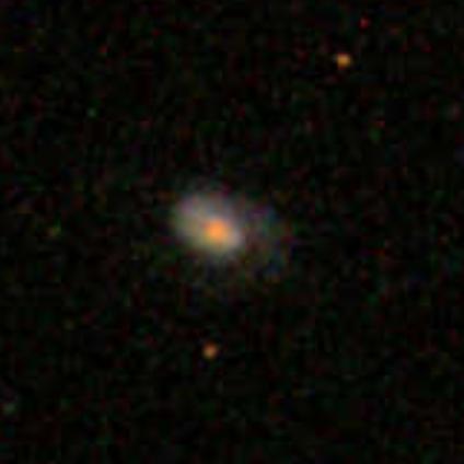
AGS00001n5, E(B-V) =
-2.07 -3.071.05, deep orange core of what may be a blue elliptical (fracDeV_g is 1 😮)1: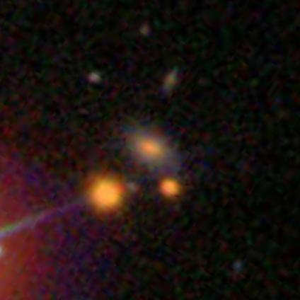
AGS00002ae, E(B-V) =
-0.84 -1.84-0.15:
AGS000003n, E(B-V) =
-0.92 -1.92-0.08
UPDATE: There were some errors in my calculation, and some of the extremes are from objects with S/N ratios, in key parameters, well below 3.
SECOND UPDATE: as I explain in a later post in this thread, I made a mistake in calculating E(B-V); the values should be (mostly) positive, and trend positive (the greater the extinction, the greater the value of E(B-V)). I am in the process of recalculating the values - using the correct formula - and have edited this post accordingly (and will edit others later).
1 It was this deeper-than-yellow color that first got me interested in tracking down dust-choked galaxies; even z~0.25 ellipticals aren't as orange as this, and the fact that the non-core parts of the galaxy seem much lighter in color, even blue in some, makes them pretty unusual in my experience (nuclei/bulges of Eos excepted, they are often yellow-tending-orange).
Posted
-
 by
trouille
scientist, moderator, admin
by
trouille
scientist, moderator, admin
Could you post where you have your E(B-V) values listed? Is it in a Dashboard or in your own computer? If on your own computer, perhaps you could copy the values into a Google spreadsheet and share the URL? It would be quite interesting to build on your work.
Posted
-
by
JeanTate
in response to trouille's comment.
Oops! 😦
Sorry Laura, I completely missed this post of yours!
It's on my own computer, and I'd gladly share it. However, the data were produced using the v2 QS catalog; now that the v3 ones (both QS and QC) are available, I'd rather re-do this work (on the QS catalog), to filter out objects with poor S/N (< 3), and add the QC ones too.
Posted
-
by
JeanTate
in response to JeanTate's comment.
In this Tools Dashboard (named "dust"; it takes a while to load) I selected QS objects with positive H-alpha, H-beta, [NII], and [OIII] line fluxes, and with S/N > 3. As I have not yet worked out how to filter on a created field, and as creating a filter for only SFR objects in a BPT diagram is, um, cumbersome, I did a very crude cut: log ([NII]/H-alpha) < -0.27. This excludes almost all the AGNs, and perhaps 2/3 of the Composite objects. I did not attempt to identify, much less remove, known outliers (e.g. AGS00001z3).
The field "EBV" is E(B-V) above, and I plotted it against
'Color' (which I guess is (u-r))(u-r) and the Sfr field (there's a wild outlier in this field!); for some reason, I can't make the plot's minimum Sfr 0.The first plot is a bit of a sanity check: the redder an object, the greater the extinction.
In the second plot, it would seem that there is a weak relationship: the dustier an object, the greater the Sfr.
UPDATE: as I explain in a later post in this thread, I made a mistake in calculating E(B-V). I have now edited the Dashboard and fixed the mistake. The correct E(B-V) values (estimates) are in the field 'EB-V'. For some reason, outliers seem more obvious; I will be investigating them later.
Posted
-
by
JeanTate
Same analysis and plots, but for QC objects in this Tools Dashboard.
It's not screamingly obvious, but comparing the EBV histogram with the QS one seems to show that a) the QS EBV distribution is wider than the QC one, and b) there is more dust - on average - in QS objects than in QC ones (assuming EBV traces dust). Some analyses of this to follow, not using Tools (you can't do direct comparisons between QS and QC in Tools).
UPDATE: as I explain in a later post in this thread, I made a mistake in calculating E(B-V). I have now edited the Dashboard and fixed the mistake. The correct E(B-V) values (estimates) are in the field 'EB-V'. For some reason, outliers seem more obvious; I will be investigating them later.
Posted
-
by
JeanTate
The four objects with the greatest E(B-V) - highest extinction/most dust - first QS then QC (number in brackets is my estimate of E(B-V)):
AGS00001sk (-3.151.15), AGS000000j (-3.111.12), AGS00001ux (-3.091.09), AGS00001n5 (-3.071.07)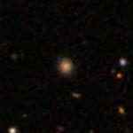
AGS00003ih (-2.980.99), AGS000044k (-2.90.90), AGS00003p8 (-2.880.89), AGS000047m (-2.860.86)
And the four with the least:
AGS00002ae (-1.84-0.15), AGS00000sl (-1.87-0.12), AGS00000hq (-1.91-0.08),AGS000000n (-1.92)AGS000003n (-0.08)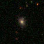
AGS00004d9 (-1.56-0.44), AGS00002pu (-1.78-0.21), AGS00004m9 (-1.83-0.16), AGS000041a (-1.88-0.12).UPDATE: as I explain in a later post in this thread, I made a mistake in calculating E(B-V); the values should be (mostly) positive, and trend positive (the greater the extinction, the greater the value of E(B-V)). I am in the process of recalculating the values - using the correct formula - and have edited this post accordingly (I have already edited several others, and will edit the remaining one(s) later). For some reason, outliers seem more obvious; I will be investigating them later.
Posted
-
by
JeanTate
in response to JeanTate's comment.
Here's the cumulative distribution function, of my estimates of E(B-V), for the SFR-dominated objects (per a BPT diagram) in the v3 QS catalog vs the v3 QC one (many thanks to mlpeck for introducing me to this technique 😃):
** IGNORE THIS ONE!! ** IGNORE THIS ONE!! IGNORE THIS ONE!! IGNORE THIS ONE!! **

-
- IGNORE THIS ONE!! ** IGNORE THIS ONE!! IGNORE THIS ONE!! IGNORE THIS ONE!! **
This is the correct CDF:

I haven't yet worked out how to find the p (probability) for a given D, in a two-tail (i.e. two empirical distributions) KS test - particularly as N(QS) != N(QC)1 - but I think it's likely to be exceedingly small. Meaning that ... QS objects are dustier than their QC counterparts.
To what extent this (fully) explains the empirical finding that QS objects are redder - as measured by (u-r) - than their QC counterparts I do not know. Nor do I know how to go about finding out.
Anyone?
1 the number of QS SFR objects is 1026; the QC number is 1068. To be selected an object needs to have an emission flux, in H-alpha, H-beta, [OIII], and [NII], > 0, AND an S/N > 3; it also needs to be in the SFR region of the BPT diagram.
UPDATE: as I explain in a later post in this thread, I made a mistake in calculating E(B-V); the values should be (mostly) positive, and trend positive (the greater the extinction, the greater the value of E(B-V)). I
am in the process ofhave finished recalculating the values - using the correct formula - and editing posts accordingly (I have already edited several others; this one is the last ... it'snot yetnow done).Posted
-
-
by
mlpeck
I think you might have something flipped, or maybe I copied down the formula incorrectly. Meaningful color excesses would be positive by the usual sign convention. I can't do a more detailed investigation at the moment but here's a dashboard with Balmer decrement excesses. E(B-V) is around 0.8-0.9 of the graphed values, and peaks around E(B-V) ≈ 0.4-0.5.
According to various sources that I'm not going to look up right now typical V band attenuation in emission line regions in the nearby universe is ~ 1 mag.
Posted
-
by
JeanTate
in response to mlpeck's comment.
Thanks! 😃
Here's my working:
E(B-V) = 0.874 * E(Hβ - Hα)
where E(Hβ - Hα) = -2.5 * log((Hα / Hβ)int / (Hα / Hβ)obs). These two come from your post, in this thread (#4, I think), which in turn come from Moustakas, Kennicutt & Tremonti (2006).Assume (Hα / Hβ)int = 2.86, per the reference you gave in post #2 (Moustakas, Kennicutt & Tremonti, 2006), then:
E(B-V) = 0.874 * -2.5 * log((Hα / Hβ)int / (Hα / Hβ)obs)
= 0.874 * -2.5 * log(2.86 / (Hα / Hβ)obs)
= -2.185 * log(2.86 / (Hα / Hβ)obs)
= -2.185 * log(2.86) + 2.185 * log(Hα / Hβ)obs)
= -0.99716 + 2.185 * log(Hα / Hβ)obs)Where did I go wrong?
UPDATE: fixed some typos and added some words
Posted
-
by
mlpeck
You just flipped the Balmer decrement -- the usual adopted value of (Hβ/Hα)int ≈ 1/2.86. I'm sure you can work out the rest.
Posted
-
by
JeanTate
in response to mlpeck's comment.
Actually, that was the typo I corrected; somehow, in my copy/pasting, I'd reversed Hβ and Hα 😛. In my spreadsheet (and dashboard) I used Hα/Hβ ... 😃
Posted
-
by
JeanTate
in response to JeanTate's comment.
Perhaps an example might help.
Take AGS000000j, which I included in a post above, giving my estimate of E(B-V) as -3.11.
I took Hαobs to be the halpha_flux field/parameter in the (QS) catalog; it has a value of 607.396. Likewise, Hβobs is hbeta_flux, which has a value of 63.0589 in the v3 catalog.
log(Hα / Hβ)obs) is thus 0.983725. And so E(B-V) is ... 1.15228. 😮
Of course, -3.11 != 1.15228; so what went wrong? mlpeck guessed right: "I think you might have something flipped"; what I'd "flipped" was the sign in front of the second term in the final equation; what I should have used was
-0.99716 + 2.185 * log(Hα / Hβ)obs)
What I actually used was
-0.99716 - 2.185 * log(Hα / Hβ)obs)
(where's the 'highly embarrassed' smilie?!?).
Now to go re-do those calculations ...
Posted
-
by
JeanTate
in response to JeanTate's comment.
I've now re-done the calculations, and edited the relevant posts in this thread accordingly (and I also re-did the two Dashboards).
mlpeck wrote:
Meaningful color excesses would be positive by the usual sign convention.
If I had known that1, I would have been more diligent, and tracked down my mistake ... before posting anything.
What, then, do the negative E(B-V) estimates mean? Some are undoubtedly the same as zero, when full error budgets are taken into account. But some are surely outliers, especially some of those in the Dashboards (not least because some of the objects are in the Composite - even AGN - part of the BPT diagram). Is there anything interesting, among these outliers?
According to various sources that I'm not going to look up right now typical V band attenuation in emission line regions in the nearby universe is ~ 1 mag.
What does "typical V band attenuation in emission line regions" mean? I'll have to find out.
here's a dashboard with Balmer decrement excesses
The Tools page launched successfully ... but everything is blank 😦 (maybe I just didn't wait long enough?).
1 In a perfect world, I would have ... I've read enough that I should have remembered that "E(B-V)" is something like "extinction, as measured by the difference between B and V flux, measured in magnitudes", and so should be > 0, as extinction is greater at shorter wavelengths (in the optical/visible part of the spectrum). Of course, there's also A(V), attenuation, etc, etc, etc. How are all these related? I don't really know, but it's surely a mini-topic of its own.
Posted
-
by
mlpeck
in response to JeanTate's comment.
The Tools page launched successfully ... but everything is blank 😦 (maybe I just didn't wait long enough?).
It's blank for me too, on two different computers. And one other dashboard I've shared does show the data and plots, at least the last time I checked. I thought this bug had been fixed. Oh well.
Posted
-
by
JeanTate
in response to JeanTate's comment.
I haven't yet worked out how to find the p (probability) for a given D, in a two-tail (i.e. two empirical distributions) KS test - particularly as N(QS) != N(QC)1 - but I think it's likely to be exceedingly small.
It seems that this probability is something you can get by plugging numbers into a 'KS two-tail test' calculator, something which is common in statistics packages. I found this online calculator; plugging my data in to that, I get (for a two-sided test):
- KS statistic: 0.27528
- P-value: 0
- Mean 1 (QS): 0.45389
- Mean 2 (QC): 0.33774
Posted
-
by
mlpeck
in response to JeanTate's comment.
Of course, there's also A(V), attenuation, etc, etc, etc. How are all these related?
My main resource for dust related jargon is a long review by Calzetti (2001). Appendix A and section 2.1, where extinction caused by a screen in front of a point source is discussed, are especially useful.
From the appendix:
The dimming effects of light are generally termed ‘extinction’ only in the simple geometrical
case of a point source behind a dust screen (section 2.1), where the attenuation suffered by the
source can be directly related to the optical depth of the dust screen.and in the next paragraph
For more general distributions of dust and emitters, the dimming and reddening of the light
is no longer directly related to the extinction or the optical depth of the dust layer, and is called
indiscriminately ‘effective extinction’, ‘obscuration’, or ‘attenuation’.Posted
-
by
JeanTate
in response to mlpeck's comment.
Thanks!
In the meantime, I'd asked a broader question on this, over in the GZ forum: Extinction, attenuation, units, physics, .... From the Calzetti paper, I learned that E(B-V) is called "the color excess", or perhaps that it's one example of a "color excess".
Posted
-
by
JeanTate
This is the E(B-V) CDF for the objects in the AGN part of the BPT diagram.
To refresh: only objects with emission line flux > 0, and S/N > 3, for all four emission lines (H-alpha, H-beta, [OIII], and [NII]) have been selected; no distinction made between AGN and LINERs. There are 546 QS "AGN" objects, and only 162 QC ones. Estimates of the color excess, E(B-V), have been calculated the same way as above.

I haven't tried to do a KS test on these distributions.
Why? Because there seem to be far too many which are unphysical.
"Unphysical"? Yes; naively, E(B-V) < 0 implies extinction/attenuation/obscuration by dust with a very unusual property: it preferentially scatters/absorbs red light! 😮 True, some of those with E(B-V) values close to 0 are likely due to inherent uncertainty (if error bars were added, they'd extend well into positive E(B-V) territory); however, there are rather a lot: ~20% of the QC objects have estimated E(B-V) < -0.05, and ~8% of the QS ones1
Of course, these rather odd results may reflect the unrealistic assumptions used to calculate E(B-V); after all, the NLRs (narrow line region) and BLRs (broad line region) surrounding the AGN accretion disk (at the heart of the QS and QC nuclei) are, physically, very different from SFRs (star-forming region). If so, how; and, more important, what difference does it make?
Perhaps these 'unphysical' E(B-V) AGNs occupy a special region in the BPT diagram? Maybe not:

Apart - perhaps - from a weak tendency for both the QS and QC 'negative E(B-V)' objects to be LINERs, and for the QC ones also to be close to the 'composite' line, there doesn't seem to be anything special about their distribution.
I looked at some of the 'negative E(B-V)' spectra (DR9 interactive) - I can't readily reproduce them here - and noticed that many (but not all) have 'observed' H-beta and H-alpha (black line) that look to me like absorption, yet the 'model' (red line) values show emission. Some examples: AGS0000322 (QC, H-beta wrong), AGS00003kj (QC, starburst, not AGN?), AGS00000vo (QS).
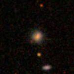
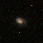
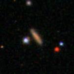
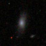
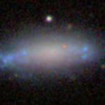
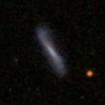
Failure of the model?At the other end - estimated E(B-V) > ~1 - there are somewhat more QC objects than among the SFRs, and very many more among the QS ones. Do these imply lots of dust? Maybe. For example AGS000000i (the first image; a QS object with E(B-V) of 1.80) seems only slightly salmon in color, while AGS00000j3 (the second; also a QS one, with E(B-V) = 1.52) is much more orange:
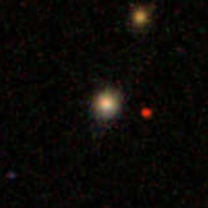
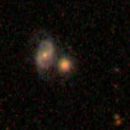
What do you think?
1 Only ~1% of the SFR QS and QC objects have estimated E(B-V) this blue
Posted
-
by
JeanTate
SCIENTIST ivywong posted a pertinent comment, on p5 of this thread: Sample Selection: Post-quenched galaxy and control galaxy :
For the dust correction, I corrected the ugriz magnitudes from the Balmer decrement using the dust models from Calzetti+00. One also has to know the E(B-V) extinction factor. I think it can be found from the published Galaxy Zoo catalogues. I'm not sure if this is true so it might be worth checking.
Basically the Calzetti model boils down to:
if (l ge 0.63 and l le 2.2) then k(i) = 2.659*(-1.857+1.040/l)+4.05
if (l lt 0.63) then k(i) = 2.659*(-2.156+1.509/l-0.198/l^2+0.011/l^3)+4.05
if (l gt 2.2) then k(i) = 0.0 where l is the wavelength in microns and k is the correction
dust_correction_factor = 10^(-0.4ebvk)
corrected_magnitude = observed_mag + 2.5 log(dust_correction_factor)I do not recall there being a "E(B-V) extinction factor" in the published Galaxy Zoo catalogs - or anywhere for that matter (for MGS SDSS galaxies, or any subset thereof) - but I'll certainly go check! 😃
Posted
-
 by
zutopian
by
zutopian
Galaxy Zoo: Dust in Spirals
We investigate the effect of dust on spiral galaxies by measuring the inclination-dependence of optical colours for 24,276 well-resolved SDSS galaxies visually classified in Galaxy Zoo.
Karen L. Masters, Robert C. Nichol, Steven Bamford, Moein Mosleh, Chris J. Lintott, Dan Andreescu, Edward M. Edmondson, William C. Keel, Phil Murray, M. Jordan Raddick, Kevin Schawinski, Anze Slosar, Alexander S. Szalay, Daniel Thomas, Jan Vandenberg
(Submitted on 12 Jan 2010 (v1), last revised 9 Feb 2010 (this version, v2))
http://arxiv.org/abs/1001.1744Posted